Abstract: Our study of 20 meteor showers revealed common characteristics of video observations between SonotaCo network (2007~2022) and GMN (2018~2023), as well as differences. While the accuracy of the determination of the radiant and geocentric velocity of the two systems was roughly equivalent, large differences were found in the measurements of meteor magnitude. The average magnitude of meteors captured by GMN is about 0.5 magnitude fainter than that of the SonotaCo network, but the scale of GMN’s magnitude estimates is narrower than that of the SonotaCo network, and the magnitude ratio calculated directly for GMN data far exceeds the value previously accepted. When comparing magnitude distributions between meteor showers, using the ratio to the sporadic meteors gives a common result for both GMN and SonotaCo network.
The characteristics of meteor showers can be clarified by the dispersion of the radiant point, the standard deviation of the geocentric velocity, the average magnitude, and the beginning and end height, and the changes in their magnitude. The following differences are the result of correcting for the effect of the geocentric velocity.
Large standard deviation of geocentric velocity: STA_SE, STA_SF, NTA.
Radiant point spreads widely: KCG, QUA, STA_SE
Many bright meteors: KCG, SPE, CAP
Many faint meteors: STA_SE, AND, ETA
High beginning height: AND, URS, low: SDA
High end height: AND, URS, CAP, low: NTA, STA_SF, STA_SE
Other special cases include NOO, which is divided into two groups based on the beginning height, and GEM, which is divided into two groups based on the magnitude distribution and the end height distribution.
Meteor showers with a small or negative difference in the beginning height compared to sporadic meteors have a high “degree of sodium depletion” according to Maeda (Maeda, 2021).
1 Introduction
We studied twenty major or interesting meteor showers using data from SonotaCo network and Global Meteor Network or GMN (Koseki, 2024b);
- April Lyrids (#006 LYR),
- eta-Aquariids (#031 ETA),
- alpha-Capricornids (#001 CAP),
- Southern delta-Aquariids (#005 SDA),
- Perseids (#007 PER),
- kappa-Cygnids (#012 KCG),
- September epsilon-Perseids (#208 SPE),
- Southern Taurids of steady expression (#002 STA_SE),
- Southern Taurids of sharply fluctuating (#002 STA_SF),
- Orionids (#008 ORI),
- Northern Taurids (#017 NTA),
- Leonids (#013, LEO),
- Andromedids (#018 AND),
- November Orionids (#250 NOO),
- December Monocerotids (#019 MON),
- sigma-Hydrids (#016 HYD),
- Geminids (#004 GEM),
- Ursids (#015 URS),
- Comae Berenicids (#020 COM)
- Quadrantids (#010 QUA).
The meteor classification is determined using our own criteria, regardless of the descriptions in the original data. For details, see Koseki, 2024a. In this paper, rather than going into the details of each meteor shower, we will use that research to compare the characteristics of observations by the SonotaCo network and GMN and also compare meteor showers with each other.
2 Characteristics of video observations: Comparison of SonotaCo network and GMN
Although both are video observations, the equipment and software used in the SonotaCo network and GMN are different. Naturally, there will be differences in the results. In this paper, we clarify the characteristics of the two by comparing the radiant points, geocentric velocities, heights of the beginning and end, and meteor magnitude of 20 meteor showers.
2.1 Geocentric velocity and its standard deviation
The geocentric velocity affects various physical quantities discussed here. First, we consider the measurement accuracy of the geocentric velocity. The standard deviation of the geocentric velocity of meteor showers clearly shows a positive correlation with the geocentric velocity, as shown in Figure 1; for information on individual meteor showers, see Table 6 at the end of this article. This increase in standard deviation indicates that the greater the geocentric velocity, the greater the error in the velocity measurement. Deviations from this overall trend are thought to be due to the inherent spatial spread of each individual meteor shower. The author divides the Taurids into three parts (Koseki, 2020); STA into early STA_SE and late STA_SF, and adds NTA to these, which he refers to as the “three Taurids” below. In Figure 1, these “three Taurids” are shown as triangles, and it is clear that they are unique. From the regression line excluding these three, it is estimated that the standard deviation of the geocentric velocity varies depending on the geocentric velocity as shown in Table 1. In the range where the geocentric velocity is small, the standard deviation of the GMN seems to be slightly smaller than that of the SonotaCo network, but the measurement error of the geocentric velocity is thought to be roughly the same for both networks over the entire region.
Table 1 – The standard deviation of the geocentric velocity estimated from the regression line excluding the “three Taurids” (triangles) in Figure 1.
| vg | 5 | 10 | 15 | 20 | 25 | 30 | 35 | 40 | 45 | 50 | 55 | 60 | 65 | 70 | |
| svg | SonotaCo | 0.77 | 0.81 | 0.84 | 0.88 | 0.92 | 0.95 | 0.99 | 1.02 | 1.06 | 1.1 | 1.13 | 1.17 | 1.21 | 1.24 |
| GMN | 0.64 | 0.69 | 0.74 | 0.79 | 0.83 | 0.88 | 0.93 | 0.98 | 1.02 | 1.07 | 1.12 | 1.17 | 1.21 | 1.26 |
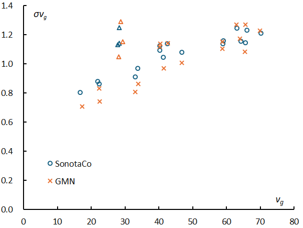
Figure 1 – Relationship between standard deviation of the geocentric velocity and geocentric velocity for 20 meteor showers.
Figure 2 shows the relationship between the geocentric velocity and the difference between the GMN and SonotaCo network (GMN–SonotaCo). STA_SF is far above the regression line, which is thought to be due to differences in the number of observations in years when its activity is active. Apart from this exception, there is a clear tendency for the GMN to have larger velocities for slow meteors and for the SonotaCo network to have larger velocities for fast meteors. This is thought to be due to differences in the method of calculating geocentric velocity and needs to be taken into consideration when considering the orbit.
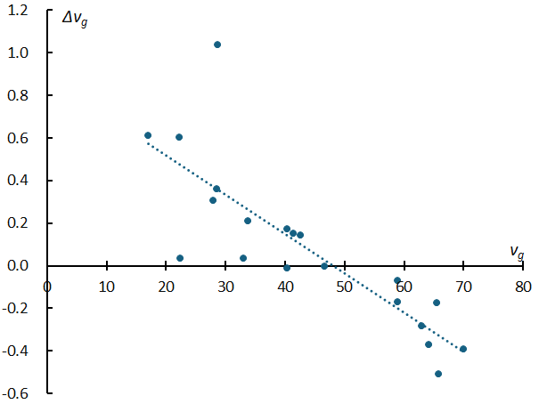
Figure 2 – Differences in geocentric velocity between the SonotaCo network and the GMN for 20 meteor showers. These are the differences in estimated values at the maximum of the meteor shower and are the value for the GMN–SonotaCo network. The point far above the regression line is STA_SF.
2.2 Spread of the radiant distribution
The spread of the radiant point is also an important indicator of the characteristics of a meteor shower. As examples of radiant point distributions obtained by the regression analysis, QUA and SDA are shown in Figures 3 and 4,
respectively by GMN. From the appearance of both, we can see that the radiant point distribution expresses the characteristics of the meteor shower. Figure 5 shows changes in the radiant point distribution density along with distance from the center for both. The vertical axis is the logarithm of the density, where the number of radiant points up to 5 degrees from the center is normalized to 1000, and shows a curve approximated by a cubic function. The difference in appearance between Figure 3 and Figure 4 can be expressed as a difference in distribution density, as shown in Figure 5. In this paper, the distance at which the radiant point density becomes one-tenth of the central radiant point density is used as a numerical value representing the spread of the radiant points and is expressed as r1/10.
Naturally, the accuracy of determining the radiant point is also expected to change depending on the geocentric velocity. It would seem that the accuracy of determining the radiant point decreases when the geocentric velocity is large, but this is not so simple.
The relationship between the distance at which the density of radiants becomes 1/10 of that at the center (the spread of radiants) and the geocentric velocity is negatively
correlated with the geocentric velocity, as shown in Figure 6; for information on individual meteor showers, see Table 6 at the end of this article. The spread of the radiant point can be estimated as Table 2 from the regression line obtained by removing the triangles in the figure where the spread of the radiant point is considered to be special (from left to right: kappa-Cygnids, Southern Taurids (STA_SE), Quadrantids. The spread of radiation points obtained from the GMN and SonotaCo networks is roughly equivalent. In addition, it is often thought that the greater the geocentric velocity, the greater the measurement error and the greater the apparent spread of the radiant point, but in fact the opposite is true.
Table 2 – The spread of the radiant points estimated from the regression line excluding the triangles shown in Figure 6.
| vg | 5 | 10 | 15 | 20 | 25 | 30 | 35 | 40 | 45 | 50 | 55 | 60 | 65 | 70 | |
| r1/10 | SonotaCo | 1.74 | 1.69 | 1.63 | 1.57 | 1.52 | 1.46 | 1.41 | 1.35 | 1.3 | 1.24 | 1.18 | 1.13 | 1.07 | 1.02 |
| GMN | 1.81 | 1.76 | 1.7 | 1.64 | 1.58 | 1.52 | 1.46 | 1.4 | 1.34 | 1.29 | 1.23 | 1.17 | 1.11 | 1.05 |
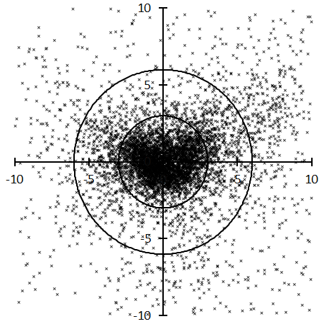
Figure 3 – The radiant distribution of the Quadrantids (QUA) after correcting radiant shift using the regression analysis by GMN.
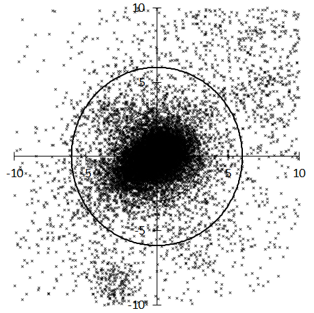
Figure 4 – Radiant distribution of the Southern delta-Aquariids (SDA) after correcting radiant shift using the regression analysis by GMN.
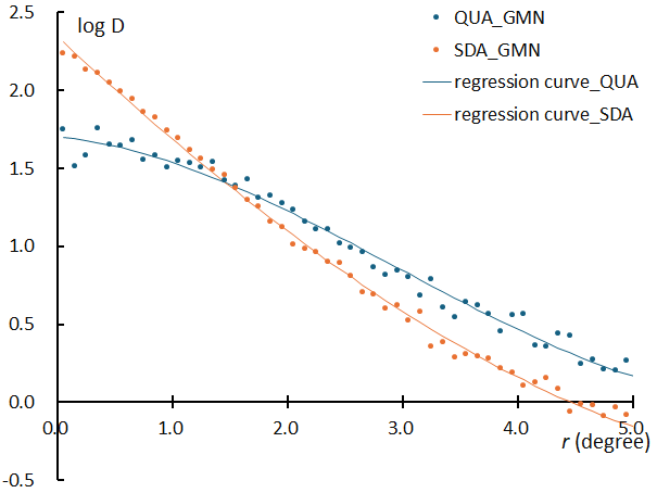
Figure 5 – Differences in radiant distribution density between the Quadrantids (QUA) and the Southern delta-Aquariids (SDA). The vertical axis is the logarithm of the density, where the number of radiant points up to 5 degrees from the center is normalized to 1000, and shows a curve approximated by a cubic function.
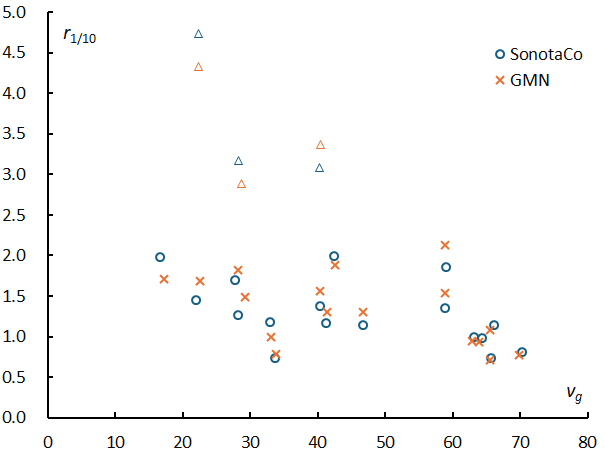
Figure 6 – The relationship between the distance at which the density of radiants becomes 1/10 of that at the center (the spread of radiants) and the geocentric velocity for 20 meteor showers. The triangles in the figure where the spread of the radiant point is considered to be special (from left to right: kappa-Cygnids, Southern Taurids (STA_SE), Quadrantids).
In order to consider the accuracy of determining the radiant point, it is necessary to consider what causes the change in the distance at which the density of the radiant points becomes one-tenth of that at the center (the spread of the radiant points).
For geometric reasons, the apparent extent of the radiant point varies greatly depending on the elongation from the Earth’s apex (εG), even if the spatial extent of the meteor shower is the same.
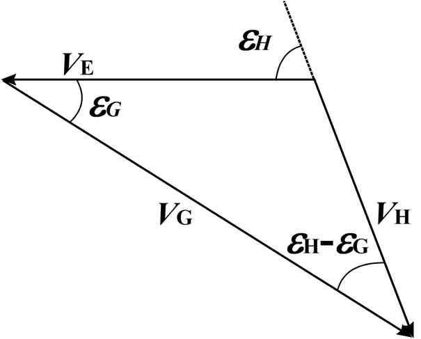
Figure 7 – Direction of motion of the meteor (vh), direction of motion of the Earth (ve), and apparent direction of motion of the meteor as seen from the Earth (vg).
The relationship between the heliocentric velocity of the meteor (vh), the Earth’s orbital velocity (ve), and the geocentric velocity of the meteor (vg) vector are expressed as shown in Figure 7. Table 3 shows the results of calculations for a meteor with a heliocentric velocity of 38 km/s, which is roughly equivalent to an ecliptic meteor shower (ANT), colliding with the Earth at various elongation angles (εh) from the Earth’s apex. When a meteoroid collides head-on with the Earth (εh = 0), the speed is vg = 68.0, but when it collides with the Earth from behind (εh = 180), the speed is much smaller at vg = 8.0. If we consider the intermediate stage, even when εh = 30, we get vg = 63.0 and εG = 16.9, so the radiant point does not appear to move very far from the Earth’s apex, and the speed does not change much. On the other hand, when εh = 170, we get εG = 138.4 and vg = 12.2, which is a large distance from the Earth’s apex. Thus, the observed angle of the meteor from the Earth’s apex (εG) does not change linearly as the direction of the meteoroid’s impact (εh) changes. dεG /dεh in Table 3 shows how εG changes with respect to changes in εh and represents the angle by which the direction of the geocentric velocity changes when the direction of the heliocentric velocity (εh) changes by 1 degree. In a geometric sense, this represents the change in the spread of the radiant point depending on the elongation of the radiant point from the Earth’s apex (εG). Even though kappa-Cygnids and Andromedids, which have εG greater than 90 degrees, have the same orbital spread as other meteor showers, the apparent spread of the radiant point to an observer on Earth is more than twice as large.
In fact, the relationship between the elongation angle of a meteor shower from the Earth’s apex (εG) and the spread of the radiant point is as shown in Figure 8, and it is clear that there is a positive correlation between the elongation angle εG from the Earth’s apex and the spread of the radiant point. The triangles in the figure indicate unusual events, and from left to right they are Quadrantids, Southern Taurids (STA_SE), and kappa-Cygnids. As shown in Table 3, the smaller the elongation εG, the larger the geocentric velocity vg. The reason why meteor showers with large geocentric velocities have a small spread is due to the geometric reason that the elongation εG is small. The negative correlation between the spread of the radiant point and the geocentric velocity is not due to observational accuracy. It would be reasonable to assume that the radiant points of slow and fast meteors are determined with roughly the same accuracy.
Table 3 – This table shows how εG and vg of a hypothetical meteor with a heliocentric velocity of 38km/s change with the change in εh in Figure 7. dεG /dεh is an index that shows the change in spread due to the elongation of the radiant point from the Earth’s apex.
| εh | 0 | 30 | 60 | 90 | 120 | 130 | 140 | 150 | 160 | 170 | 180 |
| εG | 0 | 16.8 | 33.9 | 51.7 | 71.5 | 79.2 | 87.9 | 98.7 | 113.7 | 138.4 | 180 |
| vg | 68 | 63 | 56.7 | 46.7 | 33.9 | 29.2 | 24.5 | 19.9 | 15.6 | 12.2 | 8 |
| dεG /dεh | 0.56 | 0.56 | 0.58 | 0.62 | 0.73 | 0.81 | 0.96 | 1.24 | 1.85 | 3.26 | 4.75 |
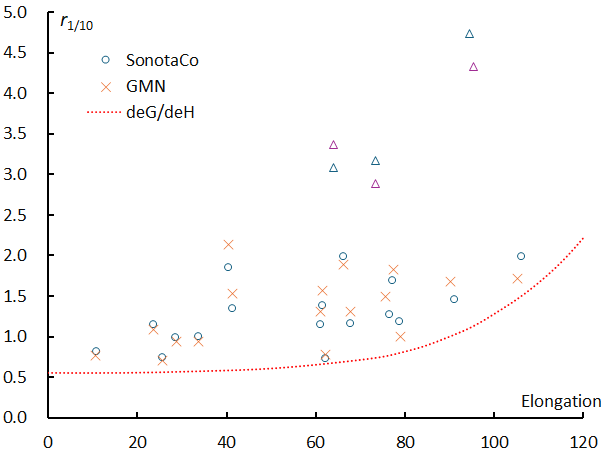
Figure 8 – The relationship between the spread of the radiants (r1/10) and the elongation from the apex of the Earth. dεG /dεh is the apparent spread of the radiants estimated from the relationship shown in Figure 7. The triangles in the figure where the spread of the radiant point is considered to be special (from left to right: Quadrantids, Southern Taurids (STA_SE), kappa-Cygnids).
When considering the spread of a meteor shower’s orbit, one should not be misled by the spread of the radiant point due to the elongation εG. It is also important to note that when the geocentric velocity is large, the observation error becomes larger, and the orbit of a meteor shower with a small elongation from the Earth’s apex εG appears to be spread out.
2.3 Magnitude of meteors
According to Öpik (1958), the mass m (g), absolute luminosity Ma and geocentric velocity v (cm/s) of a meteor are related as follows:
Various equations have been proposed by researchers to relate these physical quantities, and they differ depending on how they estimate the physical properties of meteoroids. However, if a meteoroid has the same physical characteristics, it is natural that its absolute luminosity will change depending on its geocentric speed, since the kinetic energy of the meteoroid is converted into light energy. Figure 9 shows how the absolute magnitude of meteoroids with masses of 0.1(g) and 1(g) changes with geocentric velocity using Öpik’s formula. From Figure 9, it is natural that meteor showers with a high geocentric velocity appear to have more bright meteors than meteor showers with a low geocentric velocity. It is important to note that the number of large meteoroids is different from the number of bright meteors.
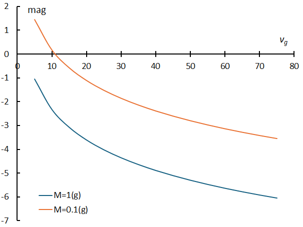
Figure 9 – Changes of the absolute magnitude of meteoroids with masses of 0.1(g) and 1(g) with geocentric velocity using Öpik’s formula.
2.3.1 Differences in meteor capture rates between the SonotaCo network and GMN due to meteor magnitude
It has been theoretically estimated that the luminosity of meteors of the same mass is a function of the geocentric velocity, and in fact, a very high correlation is observed between the average magnitude and the geocentric velocity of sporadic meteors within ±3 km/s of the geocentric velocity for the 20 meteor showers (Figure 10). The difference between the regression line shown in Figure 10 and the values of each meteor shower is an important indicator of the characteristics of the meteor shower and will be discussed in a later section.
Both the SonotaCo network observations and the GMN average magnitude show a strong correlation with the geocentric velocity, but what is most interesting in Figure 10 is that there is a large difference in the average magnitude between the two. Even with the same geocentric velocity, the average magnitude of the GMN is always higher than that of the SonotaCo network, which means that the GMN captures fainter meteors than the SonotaCo network. It has been shown that this tendency becomes stronger as the geocentric velocity decreases. This may be because the SonotaCo network uses more lenses with shorter focal lengths than the GMN, or because slow-moving light spots are excluded to avoid noise caused by light pollution. In any case, it should be noted that the GMN captures slower meteors than the SonotaCo network. Also, the difference in the slope of the regression line is related to the difference in the photometric measurements between the two, which will be discussed in the next section.
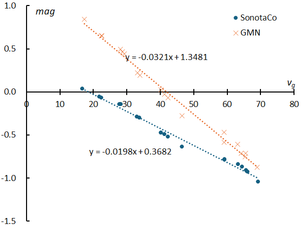
Figure 10 – The mean magnitude of sporadic meteors with geocentric velocities of ±3 km/s for 20 meteor showers.
2.3.2 Differences between SonotaCoNet and GMN photometric measurements
There is another important issue regarding meteor luminosity. The two graphs in Figures 11 and 12 compare the magnitude distributions of sporadic meteors with vg = 17~23 (km/s) and vg = 57~63 (km/s) respectively from the SonotaCo network and the GMN network. In both cases, the number of meteors is normalized to 100000, and the number of meteors per 0.1 unit of magnitude is shown in logarithm. For slow meteors (Figure 11), the extreme values of the GMN are for fainter meteors than the SonotaCo network, which shows that the GMN captures fainter meteors than the SonotaCo network. However, it is noteworthy that the GMN has an extremely low number of bright meteors. In addition, for fast meteors, the extreme values of the GMN and SonotaCo nets approach each other, and the GMN distribution is inside the SonotaCo net distribution, indicating that there is a systematic difference in the meteor luminosity measurements between the two.
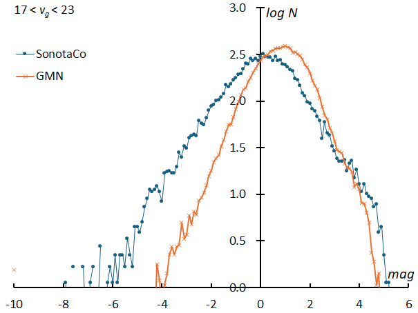
Figure 11 – The magnitude distribution of sporadic meteors with geocentric velocity 17~23km/s. The number of meteors is normalized to 100000, and the number of meteors per 0.1 unit of magnitude is shown in logarithm.
There is another important issue regarding meteor luminosity. The two graphs in Figures 11 and 12 compare the magnitude distributions of sporadic meteors with vg = 17~23 (km/s) and vg = 57~63 (km/s) respectively from the SonotaCo network and the GMN network. In both cases, the number of meteors is normalized to 100000, and the number of meteors per 0.1 unit of magnitude is shown in logarithm. For slow meteors (Figure 11), the extreme values of the GMN are for fainter meteors than the SonotaCo network, which shows that the GMN captures fainter meteors than the SonotaCo network. However, it is noteworthy that the GMN has an extremely low number of bright meteors. In addition, for fast meteors, the extreme values of the GMN and SonotaCo nets approach each other, and the GMN distribution is inside the SonotaCo net distribution, indicating that there is a systematic difference in the meteor luminosity measurements between the two.
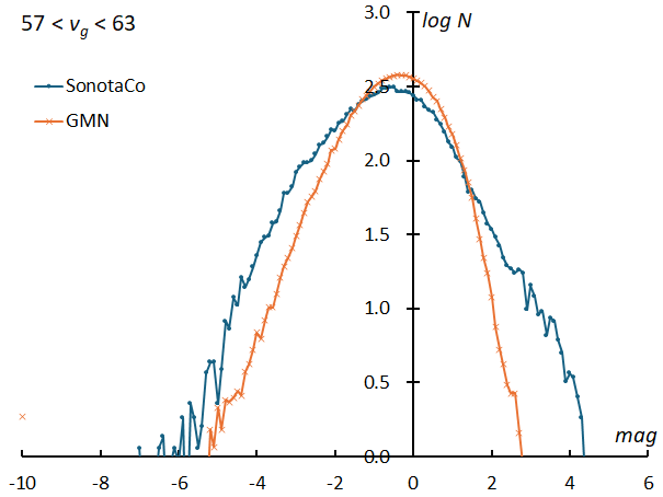
Figure 12 – The magnitude distribution of sporadic meteors with geocentric velocity 57~63km/s. The number of meteors is normalized to 100000, and the number of meteors per 0.1 unit of magnitude is shown in logarithm.
This means that there is a serious problem in directly calculating the magnitude ratio from the meteor magnitude distribution curve. Figure 13 shows the magnitude distribution of Geminids by the SonotaCo network, and Figure 14 shows GMN. The slope of the regression line obtained from the part where linear approximation is possible is 0.8560 for the SonotaCo network and 0.7861 for the GMN as shown in figures. If we calculate the magnitude ratio from these, it comes to 7.18 in SonotaCo network and 6.11 in GMN, which is far from the commonly accepted value of 2 to 3. Therefore, in this paper, we will estimate the magnitude distribution and magnitude ratio using the method described below and grasp the characteristics of the meteor shower.
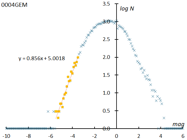
Figure 13 – The magnitude distribution of Geminids by SonotaCo network. The number of meteors is normalized to 100000, and the number of meteors per 0.1 unit of magnitude is shown in logarithm.
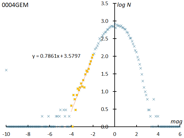
Figure 14 – The magnitude distribution of Geminids by GMN. The number of meteors is normalized to 100000, and the number of meteors per 0.1 unit of magnitude is shown in logarithm.
2.3.3 The slope of the meteor shower magnitude distribution relative to sporadic meteors
The magnitude ratio is an important indicator of the characteristics of a meteor shower, but as mentioned above, there are problems with estimating the magnitude ratio directly from the magnitude distribution. Therefore, the magnitude distribution is created by expressing the logarithm of the ratio (rsh/sp) of the number of meteors in a meteor shower to the number of sporadic meteors that have approximately the same geocentric velocity (±3 km/s from the meteor shower). Figure 15 shows the ratio of the number of meteors in Geminids to the number of sporadic meteors as a magnitude distribution for a period of 263° < λʘ < 265°, as determined by the SonotaCo network. Compared to estimating the magnitude ratio directly from the magnitude distribution shown above, we are able to obtain straight line sections that extend the range to include fainter meteors. This shows that the assumption that the oversight rate is the same for meteors of the same brightness and speed, whether they are showers or sporadic meteors, is valid.
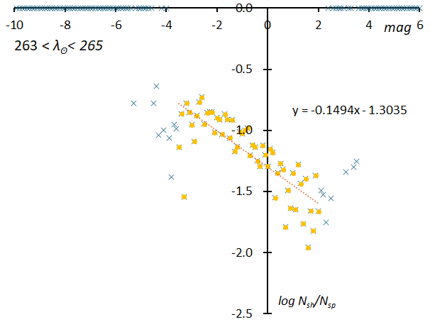
Figure 15 – The ratio of the number of meteors in Geminids to the number of sporadic meteors as a magnitude distribution for a period of 263° < λʘ < 265° by SonotaCo network. The vertical axis is a logarithmic scale.
Using this ratio (rsh/sp) also avoids the problem of differences in photometric measurements between SonotaCoNet and GMN. Figure 16 compares the slope of the magnitude distribution (rsh/sp) determined for each of the 20 meteor showers, which is roughly expressed as a straight-line y = x. This means that the slopes of the magnitude distributions (rsh/sp) obtained by the SonotaCo network and the GMN are equal.
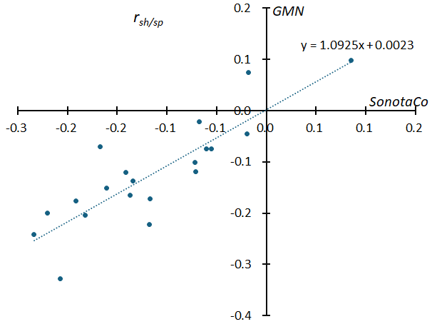
Figure 16 – The slope (rsh/sp) in Figure 15 was calculated for 20 meteor showers and compared between SonotaCo.net and GMN. Although the two use different scales for measuring meteor luminosity, this can be corrected by using rsh/sp, making it possible to compare the magnitude distribution of meteor showers.
2.3.4 The difference between the average magnitude of sporadic meteors and the average magnitude of a meteor shower
Because there are differences in the photometric measurements used by SonotaCo.net and GMN, the average magnitude of meteors cannot be used directly as an indicator of the characteristics of a meteor shower. However, the difference between the regression line shown in Figure 10 and the values of each meteor shower (Δavemag) is an important indicator of the characteristics of the meteor shower. Figure 17 is Figure 10 with the average magnitudes of 20 meteor showers as observed by GMN added. The average magnitudes of meteor showers also have a negative correlation with the geocentric velocity, but this is not as clear as in sporadic meteors, and there are considerable differences between meteor showers. Figure 18 compares these differences (Δavemag) between SonotaCo network and GMN for 20 meteor showers. Since there is a strong correlation between the two, the differences seen for each meteor shower in Figure 16 are not coincidences but are due to the characteristics of each meteor shower. The slope of the regression line in Figure 18 is approximately two-thirds of that of Figure 16 and the reason is thought to correspond to the narrower width of the magnitude distribution curves shown in Figures 11 to 14 for the GMN compared to the SonotaCo network.
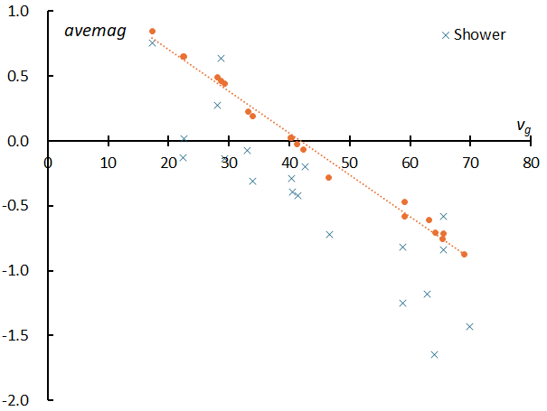
Figure 17 – The mean magnitudes of the 20 meteor showers have been added to the GMN observations in Figure 10.
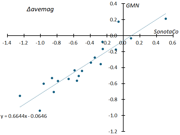
Figure 18 – The differences (Δavemag) between the regression line for sporadic meteors and the average magnitude of 20 meteor showers. Since there is a difference in the photometric measurements between the two, the slope of the regression line is smaller than that shown in Figure 16.
2.3.5 Relationship between the slope of magnitude distribution and the average magnitude
As shown in Figure 19, it is natural that the slope of the magnitude distribution of a meteor shower relative to sporadic meteors (rsh/sp) correlates with the difference in the average magnitude of the meteor shower (Δavemag). However, since there are differences in photometric measurements between the SonotaCo network and the GMN, there is a difference in the slope as can be seen in the figure. However, when considering the characteristics of a meteor shower’s magnitude distribution, it is possible to use either the slope of the relative magnitude distribution (rsh/sp) or the difference in average magnitude (Δavemag). In what follows, we will describe the characteristics of meteor showers using the difference in average magnitude (Δavemag), which is easy to understand intuitively.
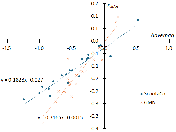
Figure 19 – A comparison of the corrected average magnitude(Δavemag) of each of the 20 meteor showers and their magnitude ratios to sporadic meteors (rsh/sp) between SonnotaCoNet and GMN.
2.4 Beginning height and end height
As shown in Figure 10, the greater the geocentric velocity, the brighter the average brightness of meteors, and so it is natural that the average beginning height will also be higher. As the beginning height becomes higher, the end height also becomes higher due to the geocentric velocity. As shown in Figure 20, as the geocentric velocity increases, the beginning (higher series) and end heights (lower series) become higher. However, it is not necessarily true that the brighter the meteor, the higher its beginning height. We will discuss this in more detail later in this section, but first we will compare the beginning heights and end heights of sporadic meteors with a magnitude of 0 between the SonotaCo network and the GMN.
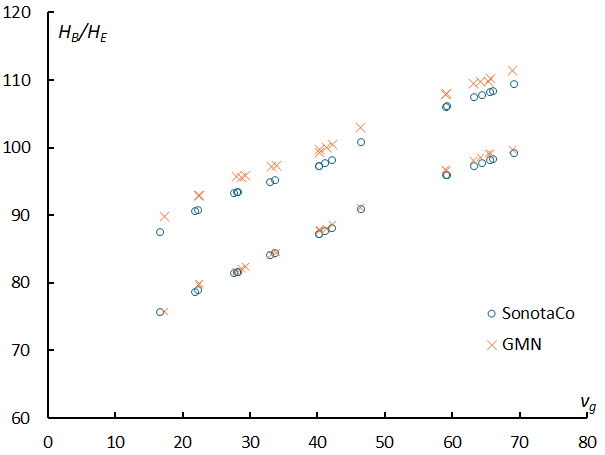
Figure 20 – The beginning height (higher series) and the end height (lower series) of sporadic meteors for magnitude 0, which have a geocentric velocity within ±3 km/s for each of the 20 meteor showers.
2.4.1 Relationship between geocentric velocity and beginning height and end height
Figure 20 shows beginning heights and end heights of sporadic meteors for magnitude 0, which have a geocentric velocity within ±3 km/s for each of the 20 meteor showers. These altitudes correspond to the intercept of the regression line for sporadic meteors shown by the dotted line in Figures 21and 22 for beginning height and Figures 25 and 26 for the end height. In both the SonotaCo network and the GMN, there is a strong correlation between the geocentric velocity and the beginning height and the end height (Figure 20). Therefore, the difference in altitude between a meteor shower and sporadic meteors indicates the characteristics of a meteor shower relative to sporadic meteors. This is touched upon in the individual sections on meteor showers (Koseki, 2024b) but will be discussed in more detail in a later section.
What is noteworthy here is that the beginning height of the GMN is always about 2 km higher than that of the SonotaCo network. On the other hand, although the difference is small, the SonotaCo network captures the end heights at lower levels. If it can track from higher to lower altitudes, this can be explained by the fact that the GMN, as mentioned earlier, can capture fainter meteors. However, this reasoning does not explain why the SonotaCo network is able to track light trails slightly lower. This is thought to be due to differences in the meteor detection methods used by the two.
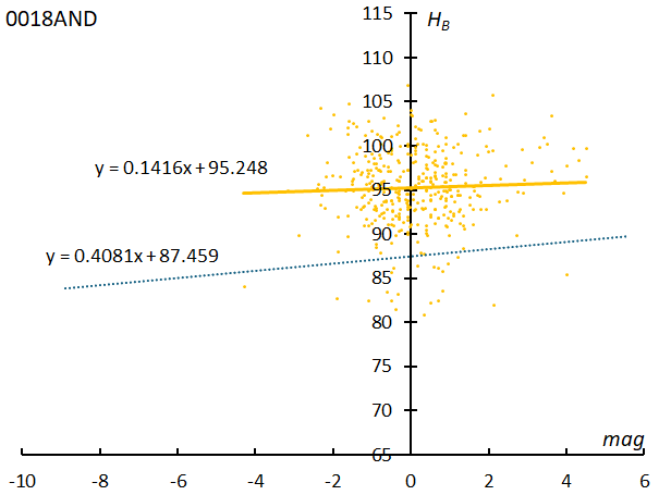
Figure 21 – The relationship between the beginning heights of Andromedids and their magnitudes by SonotaCo network. The dotted line shows the regression line for sporadic meteors.
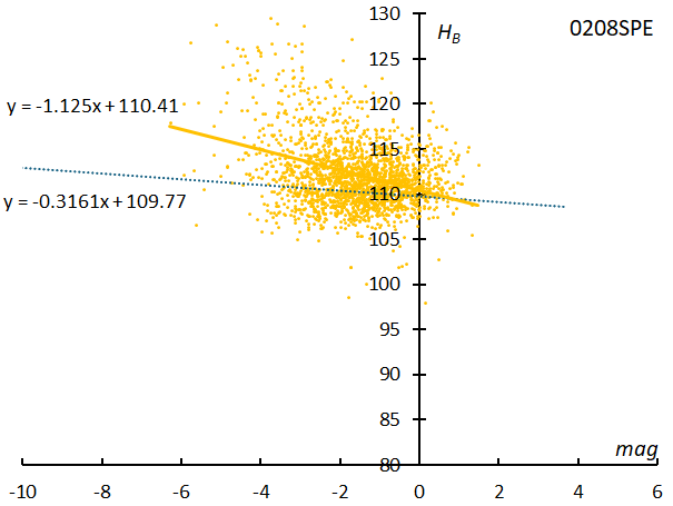
Figure 22 – The relationship between the beginning heights of September epsilon-Perseids and their magnitudes by GMN. The dotted line shows the regression line for sporadic meteors.
2.4.2 Meteor magnitude and beginning height
Figure 21 shows the relationship between the magnitude and the beginning height of the Andromedids based on observations by the SonotaCo network. The beginning height of the Andromedids is slightly higher on the fainter meteor side, with the regression line being y = 0.1415 x + 95.248. Similarly, the beginning height of sporadic meteors with a geocentric velocity of ±3 km/s from the average of the Andromedids is expressed by y = 0.4081 x +87.459, which is higher for fainter meteors. The brighter the meteor, the higher the beginning height is not always true. The slope of the regression line of the beginning height changes depending on the geocentric velocity.
For comparison with the Andromedids Figure 22 shows the relationship between the magnitude and the beginning height of the fast meteor shower September epsilon-Perseids (#208SPE), based on data from GMN. For SPE, which has a high geocentric velocity, the graph of the beginning height slopes downward to the right, which is in line with the general understanding that the brighter the meteor, the higher the beginning height. The phenomenon that the brighter the meteor, the higher its beginning height is observed in high-speed meteor showers such as Perseids and Leonids.
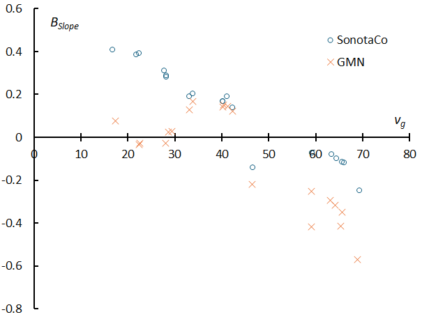
Figure 23 – The relationship between the slope of the regression line (abbreviated as BSlope) for the beginning heights of sporadic meteors and the geocentric velocity (see Figures 21&22), based on data from the SonotaCo network and GMN.
Figure 23 shows the relationship between the slope of the regression line (abbreviated as BSlope) for the beginning heights of sporadic meteors and the geocentric velocity, based on data from SonotaCo network and GMN. As already mentioned in the comparison between Andromedids and September epsilon-Perseids, the slope of the regression line (BSlope) decreases with the geocentric velocity, and what was positive (upward) becomes negative (downward). In the case of SonotaCo network, the BSlope is almost linear, whereas in the case of GMN, it rises once at a geocentric velocity of around 30 to 45 km/s and then drops sharply at the 45 km/s threshold. The boundary where the sharp decrease occurs corresponds to the boundary where the slope becomes 0 in SonotaCo network. We will discuss this boundary later, but basically, as the geocentric velocity increases, the beginning height will be lower for fainter meteors, and the slope of a graph (BSlope) will be downward sloping to the right. Further study is needed to determine whether the phenomenon in which dimmer slow meteors have higher beginning heights than brighter meteors is due to the physical properties of the meteoroid or whether it is an apparent effect of measuring the meteor luminosity.
Although the relationship is not linear, the BSlope of a sporadic meteor varies continuously with the geocentric velocity. Therefore, the difference between the BSlope of a sporadic meteor and that of a meteor shower indicates the characteristics of each meteor shower. Figure 24 shows the BSlope of meteor showers added to the SonotaCo net data in Figure 23 and shows that the BSlope of meteor showers are mostly lower than those of sporadic meteors, meaning that the BSlope-values are smaller.
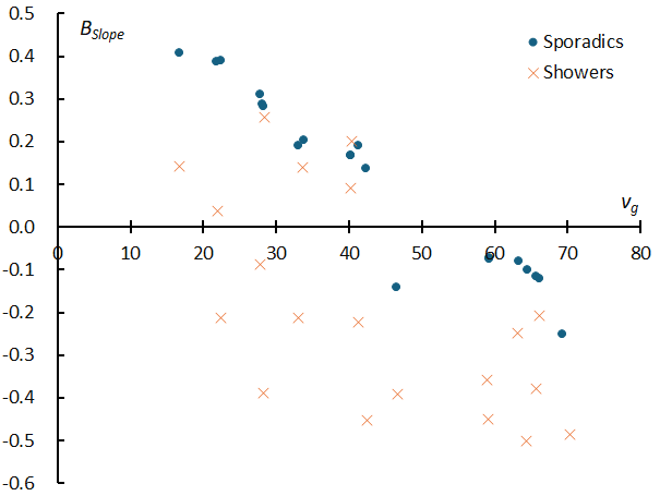
Figure 24 – The SonotaCo net data in Figure 23 with the BSlope of 20 meteor showers added.
2.4.3 Meteor magnitude and end height
As with the beginning height, the relationship between the end heights of Andromedids and their magnitude is shown based on observations by the SonotaCo network (Figure 25). In both the Andromedids and sporadic meteors, the fainter the meteor, the higher the end height, and the slope of this regression line (abbreviated as ESlope) also changes depending on the geocentric velocity, just like the beginning height.
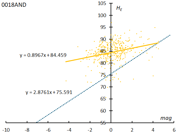
Figure 25 – The relationship between the end heights of Andromedids and their magnitudes by SonotaCo network. The dotted line shows the regression line for sporadic meteors.
For comparison with Andromedids, Figure 26 shows the relationship between the magnitude and the end height of the fast meteor shower September epsilon-Perseids (#208SPE), based on data from GMN. The slope of the graph of sporadic meteors in Figure 26 is slightly smaller than that of the Andromedid meteors (Figure 25). We can see that the slope of the end height (ESlope) also changes depending on the geocentric velocity.
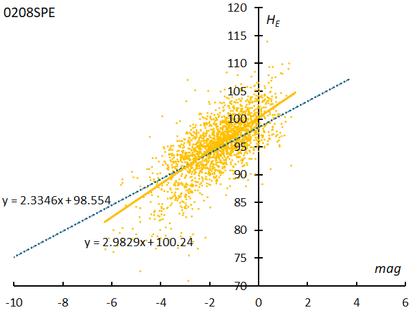
Figure 26 – The relationship between the end heights of September epsilon-Perseids and their magnitudes by GMN. The dotted line shows the regression line for sporadic meteors.
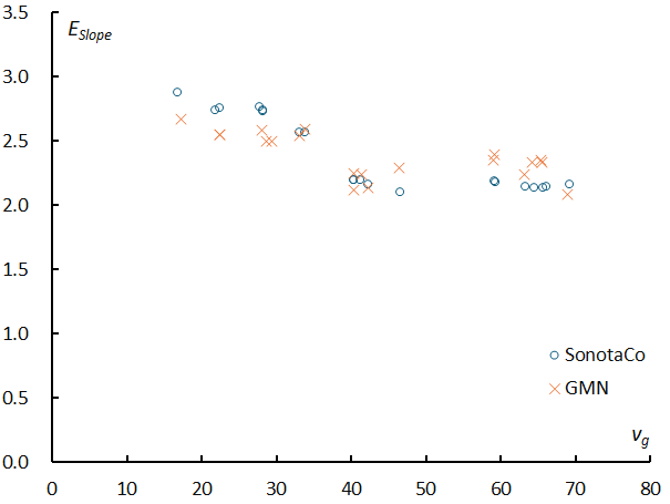
Figure 27 – The relationship between the slope of the regression line (abbreviated as ESlope) for the end heights of sporadic meteors and the geocentric velocity (see Figures 25&26), based on data from SonotaCo network and GMN.
Figure 27 shows the relationship between the slope of the regression line (ESlope) for the end heights of sporadic meteors and the geocentric velocity, based on data from the SonotaCo network and GMN. Unlike the case of the beginning height, the slope of the graph (ESlope) is always positive for the end height, the brighter the meteor, the lower the end height. The slope of the end height (ESlope) decreases with geocentric velocity but gradually becomes somewhat gentler. The relationship between ESlope and geocentric velocity is not linear but rather becomes constant from around 45 km/s, and the graph appears to be bifurcated. This boundary is also observed in the case of the beginning height and will be reconsidered below. As with the case of the beginning height, there are slight differences in the graphs between SonotaCo network and GMN.
Figure 28 shows the ESlope of meteor showers added to the SonotaCo net data in Figure 27. As we will touch on when discussing the characteristics of meteor showers, the differences in ESlope also express the individuality of each meteor shower.
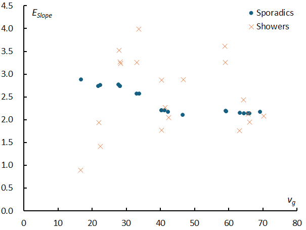
Figure 28 – The SonotaCo net data in Figure 27 with the ESlope of 20 meteor showers added.
2.4.4 Difference between beginning height and end height
When comparing the difference between the beginning height and the end height (hereinafter simply referred to as the path length) between the SonotaCo network and the GMN for sporadic meteors, the path length of GMN is about 2 km longer (Figure 29). This is due to the large influence of the difference between the beginning height of both (see Figure 20). This difference tends to shrink slightly as the geocentric velocity increases. What is more noteworthy is the step-in path length at geocentric velocities of 30 to 40 km. According to SonotaCo network, the path length is 12 km when the geocentric velocity is below 30 km/s, but is shortened to 10 km when the geocentric velocity is above 40 km/s. Here too, there exists a boundary at the geocentric velocity of 45 km/s, as seen in the BSlope and ESlope. This boundary between 40 and 45 km/s geocentric velocity is thought to be an issue related to the origin of meteors and will be discussed in the next section.
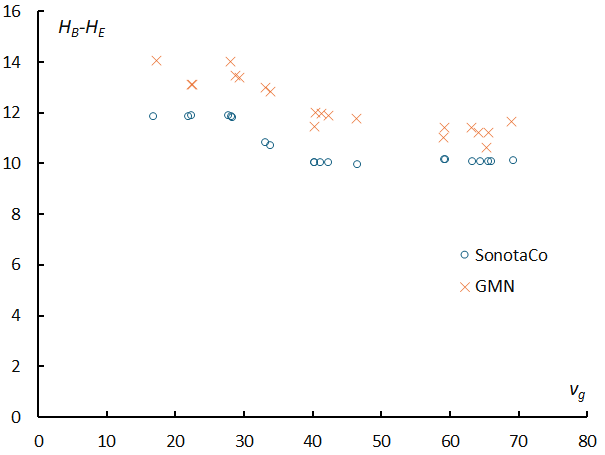
Figure 29 – The comparison of the difference between the beginning height and the end height (the path length) between SonotaCo network and GMN for sporadic meteors.
3 Characteristics of meteor showers revealed by comparing observational data
3.1 Long-period comet type and short-period comet type: orbital changes during active periods
The relationship between the elongation from the Earth’s apex and the geocentric velocity for the 20 meteor showers discussed here is shown in Figure 30. The meteor showers are divided into two groups at elongation of about 50 degrees and geocentric velocity of about 45 (km/s). This bisection occurs in all meteors and is thought to be related to their origin.
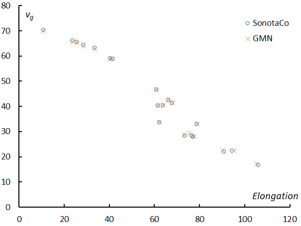
Figure 30 – The relationship between the elongation from the apex of the Earth and the geocentric velocity of the 20 meteor showers.
eta-Aquariids (#031 ETA), Perseids (#007 PER), September epsilon-Perseids (#208 SPE), Orionids (#008 ORI), Leonids (#013 LEO), sigma-Hydrids (#016 HYD), Comae Berenicids (#020 COM) form the upper left cluster in Figure 30. These have long-period comet-type (Halley type) orbits. The remaining meteor showers have short period comet-type (Jupiter family) or asteroid-type orbits. In the following, they are abbreviated as LP and SP, respectively. When comparing meteor showers, the characteristics of the showers should be considered with this basic classification in mind.
Figure 31 shows the amount of movement of the radiant point in the (λ–λʘ, β) coordinate system relative to a change of 1 degree of the solar longitude, which was calculated when creating the radiant point distribution of the meteor shower (for examples Figures 3 and 4). Figure 32 shows the absolute value of the change in the geocentric velocity for a change of 1 degree of the solar longitude, which was determined when classifying meteors to the meteor shower. The boundary for both changes is the elongation of 50 degrees from the Earth’s apex. The amount of movement of the radiant point decreases up to the elongation of 50 degrees, after which it increases. The change in geocentric velocity is almost constant up to the elongation of 50 degrees but increases thereafter. These are thought to represent differences in the intersection conditions between the meteor shower’s orbit and the Earth’s orbit. Where the amount of movement of the radiant point of a meteor shower with an elongation angle of up to 50 degrees is small in the (λ–λʘ, β) coordinate system, this is thought to be because the orbit of the meteor shower moves parallel to the Earth’s orbit, that is, the orbit rotates around the ecliptic pole. On the other hand, orbits with the elongation of 50 degrees or more tend to rotate not only around the ecliptic poles, but also around the perihelion of the meteor shower. When the direction of the perihelion and the semi-major axis of the orbit are constant and intersect with the Earth’s orbit, the movement of the radiant point in the (λ–λʘ, β) coordinate system and the change in the geocentric velocity become large.
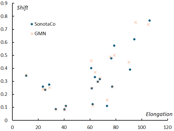
Figure 31 – The relationship between the amount of radiant shift and the elongation from the apex of the Earth. The amount is calculated in the (λ–λʘ, β) coordinate system relative to a change of 1 degree of the solar longitude, which was calculated when creating the radiant point distribution of the meteor shower.
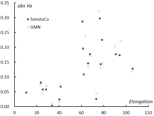
Figure 32 – The relationship between the change in the geocentric velocity and the elongation from the apex of the Earth. The change in the geocentric velocity is the absolute value for a change of 1 degree of the solar longitude, which was determined when classifying meteors to the meteor shower.
3.2 Geocentric velocity and radiant spread: orbital spread
3.2.1 Standard deviation of the geocentric velocity
Essentially, geocentric velocity is a factor in the size and shape of the orbit. Since the measurement error (standard deviation) changes depending on the geocentric velocity, it is necessary to correct this before considering the results. Figure 33 shows a comparison of the difference (Δσvg) between the regression line excluding the “three Taurids” shown in Figure 1 and the standard deviation of the geocentric velocity of each meteor shower for SonotaCoNet and GMN. The corrected spread of the geocentric velocities (Δσvg) is almost proportional between SonotaCo network and GMN. The meteor shower in the upper right of Figure 33 has a large variation in geocentric velocity, and therefore a large variation in the size and shape of its orbit. Not surprisingly, the orbital variation of the “three Taurids” is striking. Among other meteor showers, the corrected spread of the geocentric velocities Δσvg) of November Orionids and Quadrantids are slightly larger. All of the meteor showers in the upper right corner of Figure 33 are short-period meteor showers (SP), and it is thought that they are subject to large perturbations from Jupiter, which causes a large spread in their geocentric velocities.
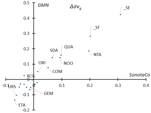
Figure 33 – The difference between the regression line excluding “three Taurids” in Figure 1 and the standard deviation of the geocentric velocity of each meteor shower.
3.2.2 Spread of the radiant points
If the geocentric velocity remains constant, the spread of the radiant point leads to a spread in the rotation of the orbital plane, i.e., the orbital inclination and the argument of perihelion. As shown in Figure 6, the spread of the radiant point correlates with the geocentric velocity. Figure 34 compares the results of SonotaCoNet and GMN by calculating the difference from the regression line excluding kappa-Cygnids, Southern Taurids (STA_SE), and Quadrantids, which deviate significantly from the correlation (see Figure 6). The two are in a nice proportional relationship, and not surprisingly, we can see that the orbits of kappa-Cygnids, Southern Taurids (STA_SE), and Quadrantids extend farther than the rest. All of these are short period (SP) meteor showers and are significantly affected by perturbations from Jupiter. Among these, the kappa-Cygnid meteor shower has a small standard deviation of its geocentric velocity despite the large spread of its radiant point. This means that although the orbital plane rotates, the size of the orbit remains nearly constant. The eta-Aquariids, Geminids, and Ursids are densely packed meteor showers with little change in orbital size, shape, and rotation.
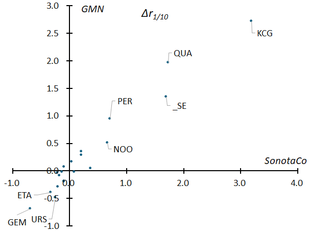
Figure 34 – The difference between the regression line excluding kappa-Cygnids, Southern Taurids (STA_SE), and Quadrantids in Figure 6 and the spread of radiants (r1/10) of each meteor shower.
3.3 Properties of meteoroids
3.3.1 Magnitude distribution of meteors
The magnitude distribution of meteors is an indicator of the mass distribution of meteoroids within a meteor shower. As shown in Figure 10, in the case of sporadic meteors, the average magnitude has an almost linear relationship to the geocentric velocity. Meteor showers, on the other hand, do have differences that are indicative of the differences in the mass distribution of meteoroids within a given shower (Figure 17).
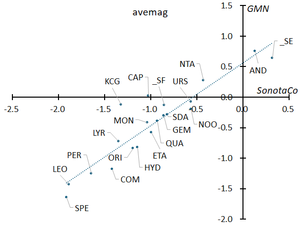
Figure 35 – The comparison of the average magnitude of meteor showers between SonotaCoNet and GMN. The differences in meteor magnitude are shown as it appears, without any correction for geocentric velocity.
Figure 35 compares the average magnitude of meteor showers between SonotaCoNet and GMN. As mentioned above, because there is a difference in the photometry between the two, the regression line does not pass through the origin and is shifted by –0.5 on the x-axis. This corresponds to the difference between the two in Figure 10.
Andromedids and Southern Taurids (STA_SE), which have positive average magnitude, have many faint meteors, while Leonids and Perseids, which have negative average magnitude, have many bright meteors. However, as seen in Figures 9 and 10, the magnitude of a meteor varies with its geocentric velocity, and unless this is corrected, the mass distribution of meteoroids in a meteor shower cannot be estimated. Figure 36 shows the difference (Δavemag) from the regression line for sporadic meteors with a geocentric velocity of ±3 km/s for each meteor shower (for an example, see Figure 17), compared between SonotaCo.net and GMN. Unlike Figure 35, the regression line passes almost through the origin because sporadic meteors are used as the comparison standard. In addition to the Southern Taurids (STA_SE), which was in the upper right of Figure 35, eta-Aquariids, which was in the middle of Figure 35, has moved to the upper right. Also, in Figure 35, alpha-Capricornids and kappa-Cygnids were in the middle, but have now moved to the lower left. By correcting for geocentric velocity, it is estimated that there are fewer high-mass meteoroids in eta-Aquariids, while conversely, there are more high-mass meteoroids in alpha-Capricornids and kappa-Cygnids.
Figure 19 shows that the mean magnitude is correlated with the magnitude distribution (rsh/sp) for sporadic meteors, and Figure 37 compares rsh/sp between SonotaCo network and GMN. From this, the relationship shown in Figure 36 can be confirmed. It is often said that fast meteor showers tend to be bright, while slow meteor showers tend to be dimmer. However, Figures 36 and 37 show that among the high-velocity meteor showers, there are some that are bright on average and have a small rsh/sp, such as Perseids and Leonids, and others that are faint, such as eta-Aquariids. Similarly, among slow meteor showers, some have many large meteoroids, such as the kappa-Cygnids and Capricornids, while others have few large meteoroids, such as Southern Taurids (STA_SE).
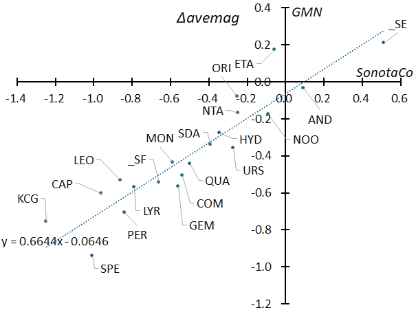
Figure 36 – This is Figure 18 with the names of meteor showers added: the difference (Δavemag) from the regression line for sporadic meteors with a geocentric velocity of ±3 km/s for each meteor shower. Since the effect of geocentric velocity has been corrected, the figure shows the mass distribution of the meteoroid rather than meteor magnitude.
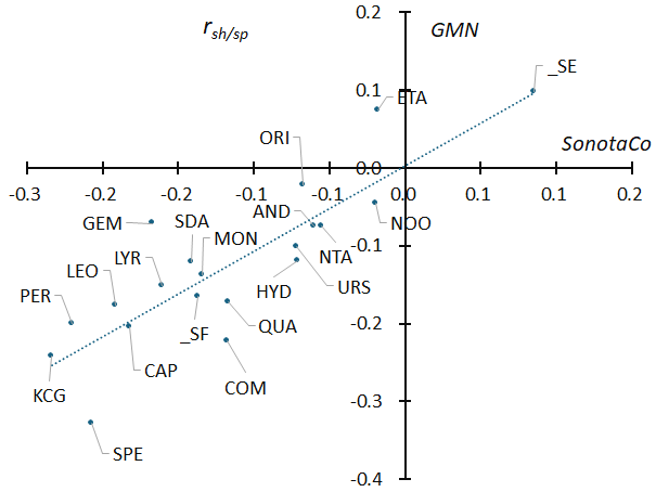
Figure 37 – This is Figure 16 with the names of meteor showers added; same as Figure 36, _SE (STA_SE: Southern Taurids) in the upper right are fainter than the sporadic meteors, while KCG (kappa-Cygnids) in the lower left are brighter.
3.3.2 Beginning height and end height
Beginning height and end height are correlated with the geocentric velocity as shown in Figure 20. Figures 38 and 39 respectively show beginning height and end height of each meteor shower, based on data from SonotaCo network. The differences from each regression line are thought to represent differences in the physical characteristics of the meteoroids in each meteor shower. The difference between the regression lines (ΔHB and ΔHE) for the SonotaCo network and GMN is compared in Figures 40 and 41, which correspond to Figures 38 and 39, respectively.
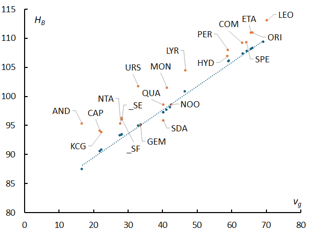
Figure 38 – Relationship between the geocentric velocity and the beginning height; meteor shower names have been added to the SonotaCo network data in Figure 20.
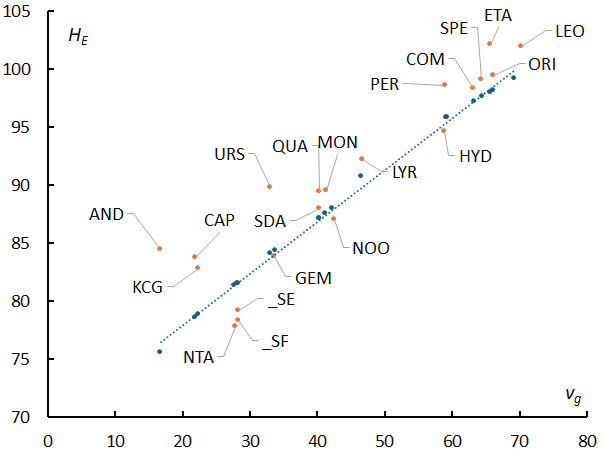
Figure 39 – Relationship between the geocentric velocity and the end height; meteor shower names have been added to the SonotaCo network data in Figure 20.
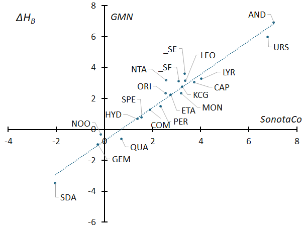
Figure 40 – The difference (ΔHB) between the regression line in Figure 38 and the beginning height of each meteor shower were calculated and compared with the (ΔHB) of GMN, which was calculated in the same way.
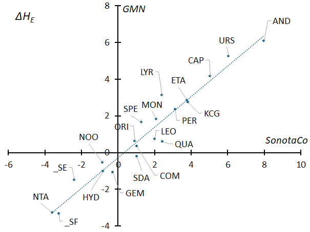
Figure 41 – The difference (ΔHE) between the regression line in Figure 39 and the end heights of each meteor shower were calculated and compared with the (ΔHE) of GMN, which was calculated in the same way.
A meteor shower with a positive difference in beginning point means that it emits light from a higher altitude than sporadic meteors with the same geocentric velocity, and a negative value means that beginning height is lower than that of sporadic meteors. Andromedids and Ursids have high beginning heights, while Southern delta-Aquariids and Geminids have slightly lower beginning heights than sporadic meteors.
The difference in the beginning points (ΔHB) is closely related to the “degree of sodium depletion” that Maeda (2021) calculated from the spectra of 2959 meteors. As shown in Figure 42, there is a clear relationship between a negative altitude difference (ΔHB) and a high degree of Na depletion, and a positive altitude difference (ΔHB) and a low degree of Na depletion. Southern delta-Aquariids and Geminids, which have lower beginning heights than the sporadic meteors, have an extremely high “degree of sodium depletion”.
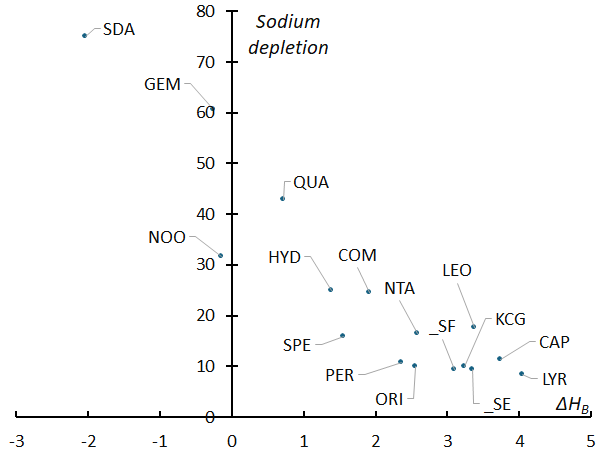
Figure 42 – The relationship between ΔHB (by SonotaCo network) and the degree of sodium depletion in meteor showers determined by Maeda (2021) using the spectra of 2959 meteors.
The specifics of the meteor shower point out that the November Orionid meteor shower (NOO) is divided into two parts based on the beginning height (Koseki, 2024b and 2025). NOO are divided into two groups: those with a beginning height of 96 km or higher and those with below 96 km. If we call the higher group NOO_H and the lower group NOO_L, then the ΔHB is 3.15 and –6.79, respectively. Extrapolating from the trends of other meteor showers, it can be inferred that the “degree of sodium depletion” of NOO_H is on par with other meteor showers, while that of NOO_L is nearly 100%.
It is quite natural that meteoroids rich in sodium begin to glow at high altitudes, while those with a high sodium depletion level are not observed until they reach an altitude where other elements such as magnesium begin to glow.
Although this is unavoidable due to the weak activity, it is unfortunate that the “degree of sodium depletion” table does not include Andromedids (AND) or Ursids (URS), which have an altitude difference (ΔHB) of 7.79 km and 6.77 km, respectively. Obtaining these spectra will enable a more reliable correlation between the difference in the beginning height (ΔHB) and the “degree of sodium depletion”. Also, December Monocerids (MON) is not included in the “degree of sodium depletion” table, presumably because it is close to NOO and therefore could not be separated. Therefore, while NOO_L has an extremely high “degree of sodium depletion”, MON, which has almost the same altitude difference (ΔHB) of 3.78 km as NOO_H, will have the same “degree of sodium depletion” as other meteor showers.
If we plot ΔHB on the horizontal axis and ΔHE on the vertical axis using GMN data (Figure 43), we can see that there is a correlation between the two, and that meteors with higher beginning height than sporadic meteors also have higher end height. Andromedids and Ursids have high beginning and end height and are estimated to be composed of fragile, sodium-rich meteoroids. Conversely, meteor showers that are closer to the origin of the coordinate system (closer to sporadic meteors), such as Southern delta-Aquariids, Geminids, November Orionids, and sigma-Hydrids, are presumed to be composed of meteoroids that are relatively resistant to fragmentation. Additionally, the “three Taurids” are unique in that their end heights are low compared to the beginning height, making them thought to be even more robust meteoroids than other meteor showers.
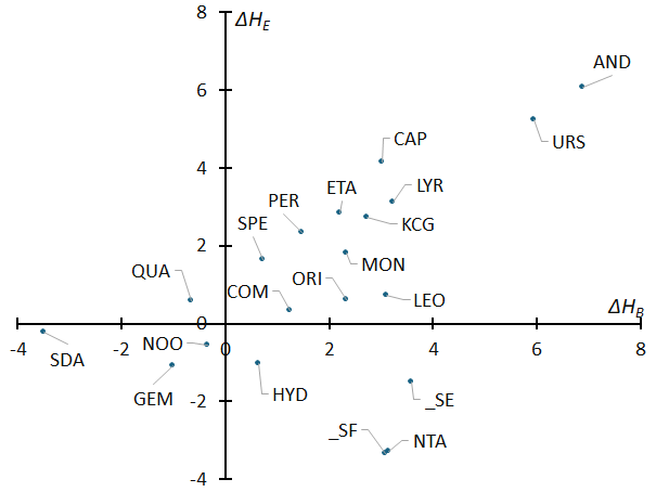
Figure 43 – The relationship between ΔHB and ΔHE based on GMN data.
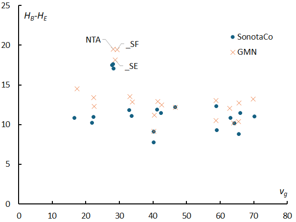
Figure 44 – The difference between the beginning height and the end height (path length) of each meteor shower against geocentric velocity.
The path lengths (the difference between the beginning height and end height) of the meteor showers are shown in Figure 44, but there are differences from those of the sporadic meteors in Figure 29. The steps seen in sporadic meteors at geocentric velocity of 35 to 40 km/s are not seen in meteor showers, and the path length remains almost constant. Of course, just as in the case of sporadic meteors, the path length is longer in GMN than in SonotaCo network in the case of meteor showers, and the difference tends to be larger for slower geocentric velocities.
What stands out in Figure 44 are the characteristics of the “three Taurids”. The “three Taurids” have path lengths nearly 5 km longer than other meteor showers. As mentioned above, this difference is due to the fact that the end heights of the “three Taurids” are lower than those of the other meteor showers; in other words, the “three Taurids” are composed of stronger meteoroids and are therefore able to penetrate lower into the atmosphere where atmospheric density is higher.
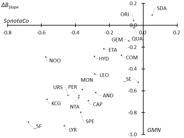
Figure 45 – The regression line of the slope (BSlope) of the beginning height against the magnitude for the sporadic meteors shown in Figure 23 was calculated, and the differences between this and the BSlope of each meteor shower were calculated.
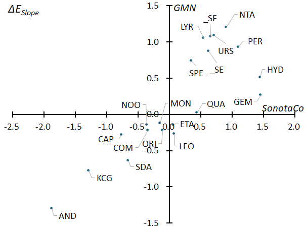
Figure 46 – The regression line of the slope (ESlope) of the end height against the magnitude for the sporadic meteors shown in Figure 27 was calculated, and the differences between this and the ESlope of each meteor shower were calculated.
As shown in Figures 24 and 28, the slope of the beginning height and the end height with respect to the geocentric velocity (BSlope and ESlope, respectively) for meteor showers are indicators that represent the characteristics of their meteoroids. A regression line is calculated for each of the slopes of the sporadic meteors in Figures 23 and 27 relative to the geocentric velocity. Figures 45 and 46 show the difference in slope (BSlope and ESlope, respectively) between sporadic meteors and each meteor shower, and compare the results between SonotaCoNet and GMN.
In Figure 45, SDA (Southern delta-Aquariids) in the upper right has a positive ΔBSlope, meaning that the rate at which the beginning height increases with meteor magnitude is greater than that of sporadic meteors, while the _SF (STA_SF: Southern Taurids) in the lower left has a negative ΔBSlope, meaning that the rate at which the beginning height decreases with meteor magnitude is greater than that of sporadic meteors.
We will explain this using Southern delta-Aquariids (SDA) in the upper right of Figure 45 and the Southern Taurids (_SF) in the lower left as examples. Southern delta-Aquariids not only have a regression line that slope upward to the right in the distribution of beginning height, but also slopes upward to the right relative to the regression line of sporadic meteors. The relationship between the two is similar to that of the regression line of Andromedids and sporadic meteors in Figure 21, but the Southern delta-Aquariids have a major different characteristic in that their regression line is lower than that of the sporadic meteors. In contrast, in Southern Taurids (_SF), the regression line slopes downward to the right compared to the regression line of the sporadic meteors. This relationship is similar to that of September epsilon-Perseids (Figure 22).
It is important to note here that the slope ESlope of the distribution of end height is basically positive (Figure 27), and the positive and negative values in Figure 46 do not represent the slope of the regression line of the end height themselves. Since the slope of sporadic meteors is used as the basis, a positive ΔESlope in the upper right corner means that the slope is steeper than the regression line of sporadic meteors, and a negative value means that the slope is shallower than the regression line of sporadic meteors.
The distribution of end height of AND in the lower left side of Figure 46 and SPE in the upper right side are shown in Figure 25 and Figure 26, respectively, so confirm the difference in ΔESlope.
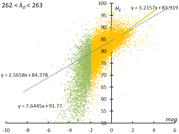
Figure 47 – The distribution of end heights of Geminids by using data of SonotaCo network for the period of 262° < λʘ < 263°.
However, further explanation is required regarding ESlope. Figure 47 shows the distribution of end heights of Geminids by using data of SonotaCo network, and there is a clear difference in the relationship between end height and magnitude at the boundary of –2 magnitude. In fact, Geminids’ bifurcation can also be seen in the magnitude distribution. Figure 15 shows the magnitude distribution of Geminids, and a clear bifurcation can be seen in the period prior to this; the magnitude distribution for the period λʘ < 263° is divided into two at magnitude –2 also. The phenomenon of the end height changing more greatly in the bright meteor region, penetrating lower, is also seen in Northern Taurids and sigma-Hydrids. Thus, path lengths tend to be longer for bright meteors than would be estimated from the mean regression line. Conversely, within the range visible to the naked eye, the path lengths of these meteor showers are shorter than those estimated from the brighter meteors. If we treat them by magnitude, it should be noted that the ΔESlope-values for these meteor showers will naturally differ from the average values shown in Figure 46, but we will not go into this further here.
Instead of a summary, a brief review of the characteristics of 20 meteor showers is given (more details see Koseki, 2024b):
April Lyrids (#006 LYR): There will be brief, sudden outbursts, and a fairly large number of bright meteors.
eta-Aquariids (#031 ETA): There are many faint meteors.
alpha-Capricornids (#001 CAP): There are many bright meteors. The end height is high. There is a tendency for the activity to become more active every year.
Southern delta-Aquariids (#005): The beginning height is low. The fainter the meteor, the higher the beginning point.
Perseids (#007): There are many bright meteors.
kappa-Cygnids (#012 KCG): The radiants are spread wide. Even bright meteors have high end heights. Activity increases every seven years.
September epsilon-Perseids (#208): There are many bright meteors.
Southern Taurids of steady expression (#002 STA_SE): Many faint meteors. Large standard deviation of geocentric velocity. Large spread of radiant point. Low end height. Long path length.
Southern Taurids of sharply fluctuating (#002 STA_SF): The standard deviation of the geocentric velocity is large. The end height is low. The path length is long. There are years when the activity is more active. In years when the activity is more active, there are many bright meteors.
Orionids (#008 ORI): During the peak activity period from 2007 to 2009, there were many bright meteors.
Northern Taurids (#017 NTA): Large standard deviation of geocentric velocity. Low end height. Long path length.
Leonids (#013, LEO): Many bright meteors. Activity is decreasing. Many meteors have geocentric velocities that deviate from the normal distribution.
Andromedids (#018 AND): Many of the meteors are dim. The beginning heights are high. Even the bright meteors have high end heights. Outburst in 2021.
November Orionids (#250, NOO): They are divided into two groups based on the beginning height. There are many faint meteors.
December Monocerotids (#019 MON): There are more bright meteors than in November Orionids
sigma-Hydrids (#016, HYD): Activity is decreasing. Bright meteors have lower end heights and shorter path lengths in the visual observation range.
Geminids (#004 GEM): The beginning height is low. Bright meteors have lower end heights. The proportion of bright meteors is low. The spread of the radiant point is small. The proportion of bright meteors increases about 0.8 days after the maximum. Based on the magnitude distribution and end heights, the meteoroids’ nature is divided into two at magnitude –2.
Ursids (#015 URS): Both the beginning height and the end height are high. There are years when the activity is more active.
Comae Berenicids (#020 COM): Their active period is extremely long, lasting from early December to mid-February.
Quadrantids (#010): The radiant point is quite spread out. The number of bright meteors increases slightly after the maximum. There are fluctuations in activity.
4 Materials
In Table 4, each meteor shower is shown in two rows, the top row is the value for SonotaCo net and the bottom row is the value for GMN. Code is the serial number and abbreviation used by the IAUMDC, and λʘ0 to β are the origin of calculation used to estimate the radiant point movement and do not represent calculation results. λʘ0 is the origin of the solar longitude, Δr is the radiant radius used for the attribution judgment, Δλʘ is the calculation range in solar longitude (Δλʘ = 5 means that the calculation used 5 degrees before and after the solar longitude given by λʘ0), and λ– λʘ and β are the initial positions of the radiant in ecliptic coordinates centered on the Sun. xa to vb are the calculation results from regression analysis. Regression analysis is performed by converting the observed position of the radiant point to (x, y) with (λ– λʘ, β) as the origin, and xa and xb are the slope a and intercept b respectively obtained when the movement of the radiant point in the x direction is expressed as x = a * λʘ + b. Similarly, ya and yb are the slope a and intercept b of the y-direction movement. va and vb are the slope a and intercept b of a similar regression analysis of the geocentric velocity. The regression analysis was repeated until convergence was achieved using only radiants within Δr degrees of the results obtained by regression analysis and radiants with geocentric velocities of ±3 km/s. “MAX” is an approximate estimate of the maximum value on the activity curve using DR15 or DR20, a moving average of 1 degree of solar longitude, and “MAX year” is the maximum percentage (%) of the meteors used to estimate the radiant point movement to the total number of meteors observed in a year; it is the maximum value on the graph showing the annual changes in the meteor shower Koseki (2024b).
In Table 5, the radiants and orbital elements are presented. These are estimated values at the maximum based on the values shown in the basic data (Table 4). λʘ is the solar longitude at the maximum, λ–λʘ to δ are the positions of the radiant point at the maximum, vg is the geocentric velocity at the maximum, e and after are the orbital elements at the maximum, λΠ and βΠ are the ecliptic coordinates in the direction of perihelion at the maximum, and last column a is the semi-major axis.
The physical characteristics of meteor showers are listed in Table 6. r1/10 is the radius at which the density of radiant points becomes 1/10 of that at the center, σvg is the standard deviation for meteors of ±3 km/s from the estimated geocentric velocity, HB and HE are the mean beginning height and end height of a magnitude 0 meteor, respectively, ΔH is the difference between the beginning height and the end height of a magnitude 0 meteor (abbreviated as the path length), ΔHB and ΔHE are the difference between the beginning height and the end height of the meteor shower and the sporadic meteor, respectively, for a magnitude 0 meteor, ΔBSlope is the difference between the BSlope of a meteor shower and the BSlope of sporadic meteors (BSlope is the slope of the regression line in the relationship between the beginning height and the magnitude of meteors), ΔESlope is also the difference between ESlopes, rsh/sp is the slope of the regression line in the range where a linear approximation is possible in the magnitude distribution, which is the logarithmic ratio of the number of meteor shower to that of sporadic meteors with roughly the same geocentric velocity (±3km/s) as the meteor shower, mag is the average magnitude of meteors classified as a member of a meteor shower, rsh and rsp are the magnitude ratios of a meteor shower and sporadic meteors with almost the same geocentric velocity (±3km/s) as the meteor shower, calculated directly from the magnitude distribution; These are only reference values, as there are large differences between the SonotaCoNet and GMN measurements of meteor brightness.
Table 4 – See explanation in Section 4.
| Code | λʘ | Δr | Δλʘ | λ–λʘ | β | xa | xb | ya | yb | va | vb | MAX | Max year |
| 0006LYR | 32 | 3 | 5 | 240.88 | 56.84 | -0.224 | 7.13 | -0.332 | 10.67 | 0.287 | 37.39 | 880 | 0.77 |
| 240.70 | 56.82 | -0.297 | 9.51 | -0.349 | 11.16 | 0.286 | 37.42 | 540 | 0.45 | ||||
| 0031ETA | 50 | 3 | 20 | 292.56 | 7.98 | 0.226 | -11.40 | 0.058 | -2.90 | 0.058 | 63.01 | 1100 | 1.98 |
| 292.61 | 7.93 | 0.228 | -11.48 | 0.059 | -2.94 | 0.043 | 63.49 | 910 | 0.72 | ||||
| 0001CAP | 125 | 2 | 10 | 179.72 | 9.54 | 0.375 | -46.70 | 0.104 | -12.90 | -0.177 | 44.44 | 230 | 0.43 |
| 179.73 | 9.59 | 0.431 | -53.81 | 0.117 | -14.64 | -0.203 | 48.03 | 135 | 0.51 | ||||
| 0005SDA | 130 | 3 | 12 | 207.62 | -7.71 | 0.221 | -28.78 | -0.108 | 14.04 | -0.195 | 65.06 | 520 | 1.32 |
| 207.53 | -7.69 | 0.221 | -28.92 | -0.109 | 14.20 | -0.195 | 65.13 | 450 | 1.15 | ||||
| 0007PER | 135 | 3 | 15 | 283.02 | 38.72 | -0.031 | 4.22 | -0.078 | 10.53 | 0.024 | 55.70 | 1500 | 10.66 |
| 283.05 | 38.68 | -0.040 | 5.47 | -0.070 | 9.53 | 0.016 | 56.58 | 1550 | 5.23 | ||||
| 0012KCG | 140 | 3 | 10 | 162.02 | 70.14 | -0.259 | 36.23 | 0.566 | -79.26 | 0.173 | -2.49 | 45 | 0.38 |
| 161.42 | 70.08 | -0.281 | 39.23 | 0.699 | -97.92 | 0.221 | -8.84 | 30 | 0.49 | ||||
| 0208SPE | 170 | 3 | 8 | 249.02 | 20.21 | -0.027 | 4.33 | -0.273 | 46.33 | 0.057 | 54.82 | 60 | 0.36 |
| 248.98 | 20.40 | 0.001 | -0.35 | -0.252 | 42.66 | 0.069 | 52.43 | 45 | 0.22 | ||||
| 0002STA_SE | 197 | 3 | 10 | 196.90 | -4.41 | 0.107 | -20.34 | -0.017 | 3.28 | -0.026 | 33.45 | 70 | 0.45 |
| 196.69 | -4.24 | 0.155 | -30.23 | -0.022 | 4.27 | -0.045 | 37.68 | 73 | 0.77 | ||||
| 0008ORI | 210 | 3 | 15 | 246.41 | -7.49 | 0.246 | -51.80 | 0.078 | -16.34 | -0.081 | 83.02 | 500 | 7.11 |
| 246.42 | -7.50 | 0.230 | -48.28 | 0.070 | -14.70 | -0.074 | 81.10 | 370 | 4.04 | ||||
| 0002STA_SF | 223 | 2 | 10 | 191.94 | -4.66 | 0.471 | -105.12 | -0.071 | 15.73 | -0.297 | 94.06 | 110 | 2.25 |
| 191.75 | -4.63 | 0.482 | -107.55 | -0.074 | 16.54 | -0.324 | 100.28 | 92 | 1.34 | ||||
| 0017NTA | 230 | 3 | 20 | 191.37 | 2.44 | 0.257 | -59.11 | 0.014 | -3.18 | -0.142 | 60.24 | 95 | 1.39 |
| 191.22 | 2.46 | 0.256 | -58.80 | 0.011 | -2.63 | -0.131 | 58.03 | 105 | 2.02 | ||||
| 0018AND | 232 | 3 | 18 | 162.14 | 22.79 | 0.446 | -103.61 | 0.624 | -144.74 | -0.127 | 46.26 | 60 | 0.32 |
| 162.29 | 23.07 | 0.443 | -102.85 | 0.590 | -136.81 | -0.120 | 44.95 | 100 | 0.48 | ||||
| 0013LEO | 237 | 3 | 10 | 271.98 | 10.07 | 0.303 | -71.72 | -0.160 | 38.01 | 0.047 | 59.23 | 180 | 2.01 |
| 272.03 | 10.05 | 0.311 | -73.74 | -0.157 | 37.26 | 0.047 | 58.64 | 110 | 0.56 | ||||
| 0250NOO | 245 | 3 | 15 | 204.28 | -7.88 | 0.290 | -71.14 | -0.054 | 13.20 | -0.145 | 78.46 | 38 | 0.58 |
| 204.34 | -7.86 | 0.290 | -70.99 | -0.059 | 14.31 | -0.134 | 75.78 | 23 | 0.52 | ||||
| 0004GEM | 255 | 3 | 10 | 208.80 | 10.86 | 0.118 | -30.20 | -0.037 | 9.41 | 0.108 | 5.37 | 2300 | 14.24 |
| 208.71 | 10.82 | 0.106 | -27.18 | -0.038 | 9.63 | 0.106 | 6.07 | 3800 | 31.79 | ||||
| 0019MON | 258 | 3 | 10 | 202.59 | -14.76 | 0.302 | -78.00 | -0.090 | 23.25 | -0.177 | 86.91 | 50 | 0.54 |
| 202.55 | -14.79 | 0.314 | -81.01 | -0.073 | 18.95 | -0.172 | 85.97 | 45 | 1.81 | ||||
| 0016HYD | 260 | 3 | 15 | 230.32 | -16.42 | 0.110 | -28.56 | -0.004 | 1.04 | -0.067 | 75.94 | 130 | 1.61 |
| 230.44 | -16.51 | 0.105 | -27.22 | -0.011 | 2.77 | -0.070 | 76.56 | 160 | 0.80 | ||||
| 0015URS | 268 | 3 | 4 | 219.68 | 70.50 | 0.097 | -25.87 | 0.565 | -151.32 | -0.225 | 93.93 | 410 | 0.46 |
| 218.02 | 70.83 | -0.102 | 27.50 | 0.489 | -131.07 | -0.146 | 72.46 | 390 | 1.01 | ||||
| 0020COM | 280 | 3 | 40 | 242.20 | 20.19 | 0.049 | -13.61 | -0.071 | 19.92 | -0.002 | 63.72 | 58 | 1.76 |
| 242.30 | 20.20 | 0.048 | -13.42 | -0.068 | 19.02 | -0.010 | 65.41 | 58 | 2.21 | ||||
| 0010QUA | 284 | 3 | 5 | 276.66 | 63.89 | 0.075 | -21.21 | 0.322 | -91.43 | -0.212 | 100.44 | 800 | 2.04 |
| 276.41 | 63.98 | 0.189 | -53.62 | 0.317 | -90.09 | -0.238 | 107.73 | 1100 | 0.53 |
Table 5 – See explanation in Section 4.
| Code | λʘ | λ–λʘ | β | α | δ | vg | e | q | i | ω | Ω | λΠ | βΠ | a |
| 0006LYR | 32.5 | 241.1 | 56.7 | 272.4 | 33.3 | 46.7 | 0.954 | 0.920 | 79.6 | 214.2 | 32.5 | 219.5 | -33.6 | 20.12 |
| 32.5 | 241.0 | 56.6 | 272.3 | 33.2 | 46.7 | 0.953 | 0.919 | 79.6 | 214.5 | 32.5 | 219.6 | -33.9 | 19.55 | |
| 0031ETA | 45.8 | 293.6 | 7.7 | 338.1 | -0.9 | 65.6 | 0.953 | 0.578 | 163.6 | 97.2 | 45.8 | 308.3 | 16.2 | 12.21 |
| 45.8 | 293.6 | 7.7 | 338.1 | -0.9 | 65.5 | 0.945 | 0.574 | 163.7 | 96.5 | 45.8 | 309.1 | 16.2 | 10.35 | |
| 0001CAP | 127.5 | 178.6 | 9.9 | 306.0 | -9.2 | 21.9 | 0.753 | 0.601 | 7.2 | 267.1 | 127.5 | 34.6 | -7.2 | 2.43 |
| 125.5 | 179.5 | 9.7 | 305.0 | -9.6 | 22.5 | 0.765 | 0.585 | 7.3 | 268.8 | 125.5 | 34.3 | -7.3 | 2.49 | |
| 0005SDA | 126.8 | 208.4 | -7.4 | 339.8 | -16.5 | 40.3 | 0.968 | 0.079 | 26.6 | 151.1 | 306.8 | 100.5 | 12.5 | 2.46 |
| 127.1 | 208.4 | -7.4 | 340.1 | -16.4 | 40.3 | 0.968 | 0.079 | 26.6 | 151.0 | 307.1 | 100.7 | 12.5 | 2.46 | |
| 0007PER | 140.1 | 283.2 | 38.4 | 48.3 | 58.0 | 59.0 | 0.938 | 0.948 | 113.1 | 150.1 | 140.1 | 332.8 | 27.3 | 15.27 |
| 140.3 | 283.3 | 38.3 | 48.8 | 58.0 | 58.8 | 0.924 | 0.946 | 113.1 | 149.6 | 140.3 | 333.2 | 27.8 | 12.51 | |
| 0012KCG | 143.5 | 164.9 | 72.1 | 287.7 | 51.0 | 22.4 | 0.698 | 0.972 | 34.3 | 205.5 | 143.5 | 345.0 | -14.1 | 3.22 |
| 141.5 | 163.0 | 71.0 | 286.5 | 49.5 | 22.4 | 0.722 | 0.970 | 33.9 | 205.9 | 141.5 | 343.5 | -14.1 | 3.49 | |
| 0208SPE | 166.9 | 249.2 | 20.9 | 47.5 | 39.5 | 64.3 | 0.960 | 0.721 | 139.2 | 245.2 | 166.9 | 288.3 | -36.4 | 17.91 |
| 166.6 | 249.2 | 21.1 | 47.1 | 39.6 | 64.0 | 0.941 | 0.718 | 138.6 | 245.9 | 166.6 | 287.4 | -37.1 | 12.20 | |
| 0002STA_SE | 200.5 | 195.7 | -4.5 | 35.4 | 9.4 | 28.3 | 0.823 | 0.307 | 5.7 | 122.3 | 20.5 | 142.9 | 4.8 | 1.73 |
| 201.5 | 195.8 | -4.4 | 36.4 | 9.8 | 28.7 | 0.830 | 0.303 | 5.7 | 122.4 | 21.5 | 144.0 | 4.8 | 1.78 | |
| 0008ORI | 209.5 | 246.7 | -7.6 | 96.3 | 15.7 | 66.1 | 0.940 | 0.570 | 163.9 | 83.2 | 29.5 | 306.5 | 16.0 | 9.50 |
| 209.3 | 246.6 | -7.6 | 96.1 | 15.8 | 65.6 | 0.917 | 0.559 | 163.8 | 85.2 | 29.3 | 304.3 | 16.1 | 6.74 | |
| 0002STA_SF | 221.5 | 192.6 | -4.6 | 52.9 | 14.4 | 28.2 | 0.829 | 0.349 | 5.4 | 115.5 | 41.5 | 157.1 | 4.9 | 2.04 |
| 219.5 | 193.5 | -4.4 | 51.7 | 14.3 | 29.3 | 0.848 | 0.327 | 5.5 | 117.5 | 39.5 | 157.1 | 4.9 | 2.15 | |
| 0017NTA | 227.5 | 192.0 | 2.4 | 56.8 | 22.4 | 27.8 | 0.823 | 0.359 | 2.8 | 294.4 | 227.5 | 161.9 | -2.5 | 2.03 |
| 227.7 | 191.8 | 2.5 | 56.7 | 22.4 | 28.1 | 0.831 | 0.358 | 2.8 | 294.0 | 227.7 | 161.7 | -2.6 | 2.12 | |
| 0018AND | 233 | 161.7 | 23.4 | 23.1 | 34.9 | 16.7 | 0.721 | 0.811 | 10.7 | 235.3 | 233.0 | 107.8 | -8.8 | 2.91 |
| 231 | 162.8 | 22.5 | 22.6 | 33.7 | 17.3 | 0.741 | 0.798 | 10.8 | 236.9 | 231.0 | 107.5 | -9.0 | 3.08 | |
| 0013LEO | 235.6 | 272.4 | 10.3 | 154.0 | 21.8 | 70.2 | 0.874 | 0.984 | 162.1 | 172.3 | 235.6 | 62.9 | 2.3 | 7.80 |
| 236.5 | 272.2 | 10.1 | 154.6 | 21.4 | 69.8 | 0.835 | 0.985 | 162.3 | 172.9 | 236.5 | 63.2 | 2.1 | 5.96 | |
| 0250NOO | 247.7 | 203.5 | -8.0 | 91.2 | 15.4 | 42.5 | 0.991 | 0.119 | 23.8 | 140.0 | 67.7 | 210.2 | 15.0 | 12.73 |
| 247.5 | 203.5 | -8.0 | 91.1 | 15.4 | 42.6 | 0.992 | 0.118 | 24.0 | 140.2 | 67.5 | 210.3 | 15.1 | 13.98 | |
| 0004GEM | 262.1 | 208.0 | 10.5 | 113.6 | 32.3 | 33.7 | 0.887 | 0.147 | 22.6 | 324.0 | 262.1 | 228.3 | -13.0 | 1.30 |
| 261.9 | 208.0 | 10.5 | 113.3 | 32.3 | 33.9 | 0.889 | 0.146 | 22.9 | 324.1 | 261.9 | 228.2 | -13.2 | 1.32 | |
| 0019MON | 257.9 | 202.6 | -14.8 | 100.3 | 8.3 | 41.3 | 0.981 | 0.183 | 35.3 | 130.0 | 77.9 | 213.7 | 26.2 | 9.61 |
| 258.1 | 202.5 | -14.8 | 100.4 | 8.3 | 41.5 | 0.984 | 0.184 | 35.4 | 129.8 | 78.1 | 213.7 | 26.5 | 11.19 | |
| 0016HYD | 254.8 | 231.0 | -16.4 | 124.2 | 2.9 | 58.9 | 0.985 | 0.256 | 129.4 | 119.5 | 74.8 | 303.1 | 42.3 | 16.72 |
| 254.5 | 231.0 | -16.4 | 123.9 | 2.9 | 58.8 | 0.983 | 0.256 | 129.3 | 119.6 | 74.5 | 302.7 | 42.3 | 14.74 | |
| 0015URS | 270.5 | 218.8 | 72.0 | 219.0 | 75.4 | 33.0 | 0.809 | 0.939 | 52.8 | 205.9 | 270.5 | 106.9 | -20.4 | 4.91 |
| 270.4 | 218.5 | 72.0 | 219.2 | 75.5 | 33.1 | 0.815 | 0.940 | 52.7 | 205.8 | 270.4 | 106.7 | -20.3 | 5.07 | |
| 0020COM | 268.1 | 242.8 | 21.0 | 161.5 | 30.6 | 63.1 | 0.959 | 0.560 | 134.4 | 263.1 | 268.1 | 7.9 | -45.2 | 13.55 |
| 267.9 | 242.9 | 21.1 | 161.4 | 30.7 | 62.9 | 0.944 | 0.558 | 134.2 | 263.8 | 267.9 | 6.7 | -45.5 | 10.00 | |
| 0010QUA | 283.2 | 276.7 | 63.7 | 229.9 | 49.7 | 40.3 | 0.627 | 0.979 | 70.8 | 171.9 | 283.2 | 100.5 | 7.7 | 2.63 |
| 283.2 | 276.7 | 63.7 | 229.9 | 49.7 | 40.4 | 0.640 | 0.980 | 71.0 | 172.0 | 283.2 | 100.6 | 7.6 | 2.72 |
Table 6 – See explanation in Section 4.
| Code | r1/10 | σvg | HB | HE | HB-HEsh | ΔHB | ΔHE | ΔBSlope | ΔESlope | rsh/sp | avemag | rsh | rsp |
| 0006LYR | 1.15 | 1.08 | 104.4 | 92.2 | 12.2 | 3.6 | 1.4 | -0.46 | 0.54 | -0.161 | -1.34 | 3.00 | 3.97 |
| 1.31 | 1.01 | 105.7 | 93.5 | 12.2 | 2.8 | 2.4 | -0.92 | 1.05 | -0.151 | -0.72 | 4.94 | 5.89 | |
| 0031ETA | 0.74 | 1.14 | 110.9 | 102.1 | 8.8 | 2.8 | 4.1 | -0.23 | 0.06 | -0.018 | -0.99 | 3.65 | 4.22 |
| 0.71 | 1.08 | 112.4 | 102.0 | 10.4 | 2.6 | 2.9 | -0.22 | -0.14 | 0.075 | -0.58 | 6.19 | 4.46 | |
| 0001CAP | 1.45 | 0.88 | 94.0 | 83.8 | 10.2 | 3.5 | 5.2 | -0.32 | -0.76 | -0.182 | -1.03 | 1.74 | 2.97 |
| 1.68 | 0.74 | 95.8 | 83.5 | 12.3 | 2.8 | 3.6 | -0.69 | -0.28 | -0.204 | 0.02 | 4.02 | 3.77 | |
| 0005SDA | 1.38 | 1.09 | 95.7 | 88.0 | 7.7 | -1.5 | 0.9 | 0.05 | -0.66 | -0.142 | -0.82 | 3.86 | 3.82 |
| 1.57 | 1.12 | 96.5 | 87.3 | 9.2 | -2.8 | -0.5 | 0.09 | -0.64 | -0.120 | -0.29 | 8.15 | 7.39 | |
| 0007PER | 1.85 | 1.16 | 107.9 | 98.6 | 9.3 | 1.9 | 2.8 | -0.38 | 1.10 | -0.220 | -1.64 | 5.33 | 4.91 |
| 2.13 | 1.15 | 109.1 | 98.6 | 10.5 | 1.2 | 1.8 | -0.65 | 0.93 | -0.200 | -1.25 | 3.06 | 4.41 | |
| 0012KCG | 4.74 | 0.86 | 93.7 | 82.8 | 10.9 | 3.0 | 3.9 | -0.57 | -1.28 | -0.234 | -1.32 | — | 3.03 |
| 4.33 | 0.83 | 95.4 | 82.0 | 13.4 | 2.5 | 2.2 | -0.68 | -0.78 | -0.242 | -0.13 | 2.32 | 3.69 | |
| 0208SPE | 0.98 | 1.16 | 109.2 | 99.1 | 10.1 | 1.5 | 1.5 | -0.37 | 0.35 | -0.207 | -1.91 | 4.05 | 4.73 |
| 0.94 | 1.17 | 110.4 | 100.2 | 10.2 | 0.6 | 1.7 | -0.80 | 0.74 | -0.328 | -1.65 | 3.20 | 5.12 | |
| 0002STA_SE | 3.18 | 1.25 | 96.2 | 79.2 | 17.0 | 2.9 | -2.3 | -0.03 | 0.62 | 0.085 | 0.32 | 2.06 | 3.50 |
| 2.88 | 1.29 | 98.8 | 80.7 | 18.2 | 3.2 | -1.5 | -0.52 | 0.87 | 0.098 | 0.64 | 4.70 | 4.27 | |
| 0008ORI | 1.14 | 1.23 | 110.9 | 99.5 | 11.4 | 2.6 | 1.3 | -0.05 | -0.11 | -0.068 | -1.19 | 4.27 | 4.37 |
| 1.08 | 1.27 | 112.6 | 99.9 | 12.7 | 2.3 | 0.8 | 0.04 | -0.22 | -0.022 | -0.84 | 4.36 | 3.51 | |
| 0002STA_SF | 1.27 | 1.14 | 96.0 | 78.4 | 17.6 | 2.6 | -3.1 | -0.67 | 0.66 | -0.137 | -0.85 | 2.89 | 3.51 |
| 1.49 | 1.15 | 98.6 | 79.2 | 19.4 | 2.8 | -3.3 | -0.89 | 1.07 | -0.165 | -0.14 | 2.43 | 4.02 | |
| 0017NTA | 1.70 | 1.13 | 95.3 | 77.8 | 17.5 | 2.1 | -3.5 | -0.38 | 0.91 | -0.055 | -0.43 | 2.77 | 3.40 |
| 1.83 | 1.05 | 98.2 | 78.6 | 19.5 | 2.5 | -3.0 | -0.67 | 1.20 | -0.074 | 0.27 | 2.46 | 3.25 | |
| 0018AND | 1.98 | 0.80 | 95.2 | 84.5 | 10.8 | 7.8 | 8.9 | -0.28 | -1.88 | -0.061 | 0.13 | — | 3.13 |
| 1.72 | 0.71 | 97.5 | 83.0 | 14.5 | 7.7 | 7.3 | -0.62 | -1.30 | -0.075 | 0.75 | 10.20 | 3.32 | |
| 0013LEO | 0.81 | 1.21 | 113.0 | 102.0 | 11.0 | 3.7 | 2.8 | -0.28 | 0.08 | -0.192 | -1.88 | 3.62 | 5.34 |
| 0.77 | 1.23 | 114.7 | 101.5 | 13.2 | 3.3 | 1.7 | -0.45 | -0.27 | -0.176 | -1.43 | 3.63 | 3.72 | |
| 0250NOO | 1.99 | 1.14 | 98.5 | 87.0 | 11.4 | 0.4 | -1.0 | -0.57 | -0.36 | -0.019 | -0.56 | 4.47 | 3.49 |
| 1.88 | 1.14 | 100.4 | 87.9 | 12.5 | 0.0 | -0.6 | -0.29 | -0.15 | -0.045 | -0.20 | 5.32 | 6.85 | |
| 0004GEM | 0.74 | 0.97 | 94.9 | 83.8 | 11.1 | -0.2 | -0.6 | -0.08 | 1.46 | -0.167 | -0.86 | 7.18 | 4.02 |
| 0.78 | 0.86 | 96.3 | 83.5 | 12.8 | -1.0 | -1.0 | -0.15 | 0.26 | -0.070 | -0.31 | 6.11 | 3.99 | |
| 0019MON | 1.16 | 1.05 | 101.4 | 89.5 | 11.9 | 3.8 | 1.9 | -0.36 | -0.15 | -0.134 | -1.04 | 3.27 | 4.04 |
| 1.30 | 0.97 | 102.7 | 89.8 | 12.9 | 2.7 | 1.8 | -0.59 | -0.12 | -0.137 | -0.42 | 3.88 | 6.30 | |
| 0016HYD | 1.35 | 1.14 | 106.9 | 94.6 | 12.3 | 0.9 | -1.2 | -0.29 | 1.45 | -0.071 | -1.14 | 4.31 | 4.89 |
| 1.53 | 1.10 | 108.3 | 95.3 | 13.0 | 0.3 | -1.3 | -0.29 | 0.51 | -0.119 | -0.82 | 4.81 | 5.52 | |
| 0015URS | 1.18 | 0.91 | 101.7 | 89.8 | 11.8 | 6.8 | 5.8 | -0.44 | 0.72 | -0.072 | -0.56 | 2.30 | 3.60 |
| 1.00 | 0.81 | 103.0 | 89.5 | 13.5 | 5.9 | 5.4 | -0.64 | 1.09 | -0.102 | -0.07 | 4.38 | 3.64 | |
| 0020COM | 1.00 | 1.25 | 109.1 | 98.3 | 10.8 | 1.8 | 1.1 | -0.13 | -0.34 | -0.117 | -1.42 | 4.37 | 4.87 |
| 0.94 | 1.27 | 110.5 | 98.5 | 12.0 | 1.0 | 0.4 | -0.28 | -0.22 | -0.223 | -1.18 | 4.38 | 3.55 | |
| 0010QUA | 3.08 | 1.12 | 98.5 | 89.4 | 9.1 | 1.3 | 2.3 | -0.05 | 0.44 | -0.117 | -0.93 | 4.88 | 3.91 |
| 3.37 | 1.14 | 99.4 | 88.2 | 11.2 | -0.3 | 0.5 | -0.03 | 0.02 | -0.172 | -0.40 | 5.53 | 5.95 |
Acknowledgments
The author expresses his deep gratitude to the SonotaCoNet (SonotaCo, 2009) and GMN observers Vida et al., 2019; 2020; 2021), without whose hard work and continued efforts, and without their generous sharing, this article would not exist.
References
Koseki M. (2020). “Three components of ‘Taurids’ II”. WGN, the Journal of the IMO, 48, 36–46.
Koseki M. (2024a). “Meteor shower data from video observation, Part I, Research methods and summary of survey results”. eMetN Meteor Journal, 9, 166–183.
Koseki (2024b). “20 meteor showers explored through video observations”. published as a series of 6 volumes by February 2025 (in Japanese).
Koseki M. (2025). “November Orionids (#250 NOO) are special”. Ssubmitted to WGN, the Journal of the IMO.
Maeda K. (2021). “Summary of meteor spectrum observations using 4K video for 5 years from 2015”, Presentation at the 3rd Meteor Spectral Conference on web (in Japanese).
Öpik E. J. (1958). Physics of Meteor Flight in the Atmosphere. Interscience, New York.
SonotaCo (2009). “A meteor shower catalog based on video observations in 2007-2008”. WGN, the Journal of the IMO, 37, 55–62.
SonotaCo (2016). “Observation error propagation on video meteor orbit determination”. WGN, Journal of the International Meteor Organization, 44, 42–45.
SonotaCo (2017). “Exhaustive error computation on 3 or more simultaneous meteor observations”. WGN, Journal of the International Meteor Organization, 45, 95–97.
SonotaCo, Masuzawa T., Sekiguchi T., Miyoshi T., Fujiwara Y., Maeda K., Uehara S. (2021). “SNMv3: A Meteor Data Set for Meteor Shower Analysis”. WGN, the Journal of the IMO, 49,64–70.
Vida D., Gural P., Brown P., Campbell–Brown M., Wiegert P. (2019). “Estimating trajectories of meteors: an observational Monte Carlo approach – I. Theory”. Monthly Notices of the Royal Astronomical Society, 491, 2688–2705.
Vida D., Gural P., Brown P., Campbell–Brown M., Wiegert P. (2020). “Estimating trajectories of meteors: an observational Monte Carlo approach – II. Results”. Monthly Notices of the Royal Astronomical Society, 491, 3996–4011.
Vida D., Šegon D., Gural P. S., Brown P. G., McIntyre M. J. M., Dijkema T. J., Pavletić L., Kukić P., Mazur M. J., Eschman P., Roggemans P., Merlak A., Zubrović D. (2021). “The Global Meteor Network – Methodology and first results”. Monthly Notices of the Royal Astronomical Society, 506, 5046–5074.