Abstract: In this article I would like to introduce a method that detects meteor echoes based on artificial intelligence. The advantages over conventional object detection are significant:
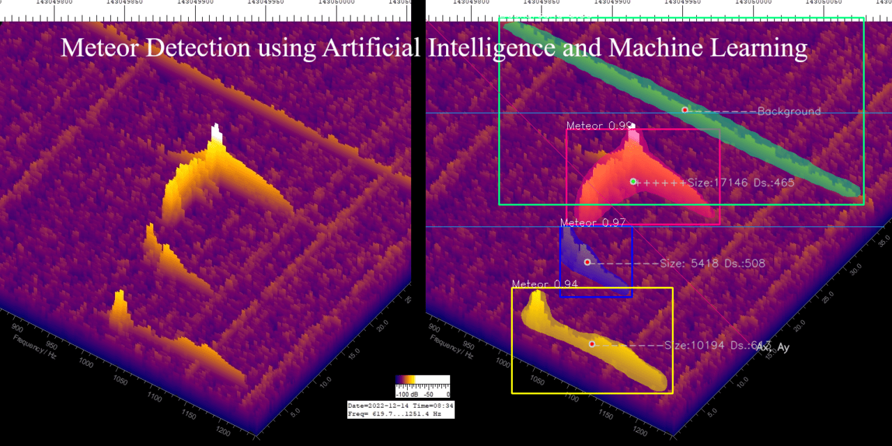
- The current version can detect meteors of various shapes and distinguish them from interferences and Starlink satellites.
- Echoes that are smaller than the interference level can be detected.
- Because there is no threshold, more echoes are detected than with the conventional method.
- The software also detects echoes that are incomplete for example due to the periodic switching process of the GRAVES antennas.
- A neural network is easy to expand or adapt to new spectrograms or emerging disturbances.
1 Introduction
For some time now I have been developing programs that record and evaluate meteor echoes. Originally it was a real-time version running on a Nvidia-Jetson-Nano-computer. Some time ago I ported the program to Windows 10 and switched to post-processing (Sicking, 2022a, 2022b). The program works well, but has flaws. Traditionally programmed object recognition is never perfect. Detection is inflexible and complicated when high accuracy is desired. Especially when many signals are in the image, echoes are missed. The data often has to be checked manually. Starlink satellites and interferences are constantly increasing. I’m also particularly interested in small echoes to examine the In-Line-Peak (Sicking, 2022a) in more detail. To increase accuracy, I looked for a way to learn to use artificial intelligence (AI) / machine learning (ML) and came across a tutorial and excellent software: The PixelLib by Ayoola Olafenwa (Olafenwa, 2020). Pixellib is a program library that provides all the procedures needed for object recognition using AI methods. The instance segmentation with PixelLib used in this work is based on the MaskRCNN framework (He et al., 2018).
In this article I would like to show how the program package works, how it is basically installed and what results come out compared to my traditional method.
2 Setup
A circularly polarized 4-element cross-Yagi antenna is used to receive the meteor echoes. My antennas are mounted in the attic so the configuration can be easily changed. A low-noise preamplifier with a frequency range of 140-150 MHz and a noise figure of 0.25 dB is connected directly to the antenna. The receiver is an Icom IC-R8600. Spectrum-Lab (SL) from Wolfgang Buescher (DL4YHF) is used as recording software. SL generates plots at 20 second intervals with corresponding date and time in the filename, which are later analysed using the software described here. For recording and programming, I use Windows 11 notebooks with i3 or i5 processors. To train the neural network, I use a Windows 10 gaming PC, also with an i5 processor and a GeForce RTX-3060 graphics card (GPU). The GPU has 3840 CUDA cores. This GPU and the corresponding Nvidia software lead to significant acceleration, especially when training the neural network. A bench test is shown below.
3 Setup of the Neural Network
Pixellib is well documented on the Internet, so only the things that are important to the project are described here.
Before you can start examining objects with AI, a neural network for the objects to be recognized, a model, must be created. Typically, an existing model is retrained. This process is called transfer learning. The Pixellib author used the mask_rcnn_coco model for this. It recognizes pretty much everything we encounter every day. An example of using mask_rcnn_coco is shown below. In her Pixellib tutorial, Ayoola Olafenwa has now retrained this model on two new objects, namely butterflies and squirrels. These two so-called classes are not included in mask_rcnn_coco and are therefore suitable for demonstrating transfer learning.
I followed the tutorial and have now retrained the mask_rcnn_coco model with three new classes. My corresponding line in the training script is:
segment_image.inferConfig(num_classes= 3, class_names= [“BG”, “Artificial-Star”, “Background”, “Meteor”])
The first BG belongs to Pixellib. Then my three classes follow.
The classes must be in ascending alphabetical order, otherwise mismatches will occur. The files in my Test and Train folders also start with A, B and the rest are for meteors.
Labeling the Data for the Three Classes
The main work now consists of collecting images of the three classes Artificial-Stars, Background and Meteor and preparing them for training the model. So far there are over 600 plots that had to be individually labeled by hand. This process is explained for Meteors based on Figure 1.
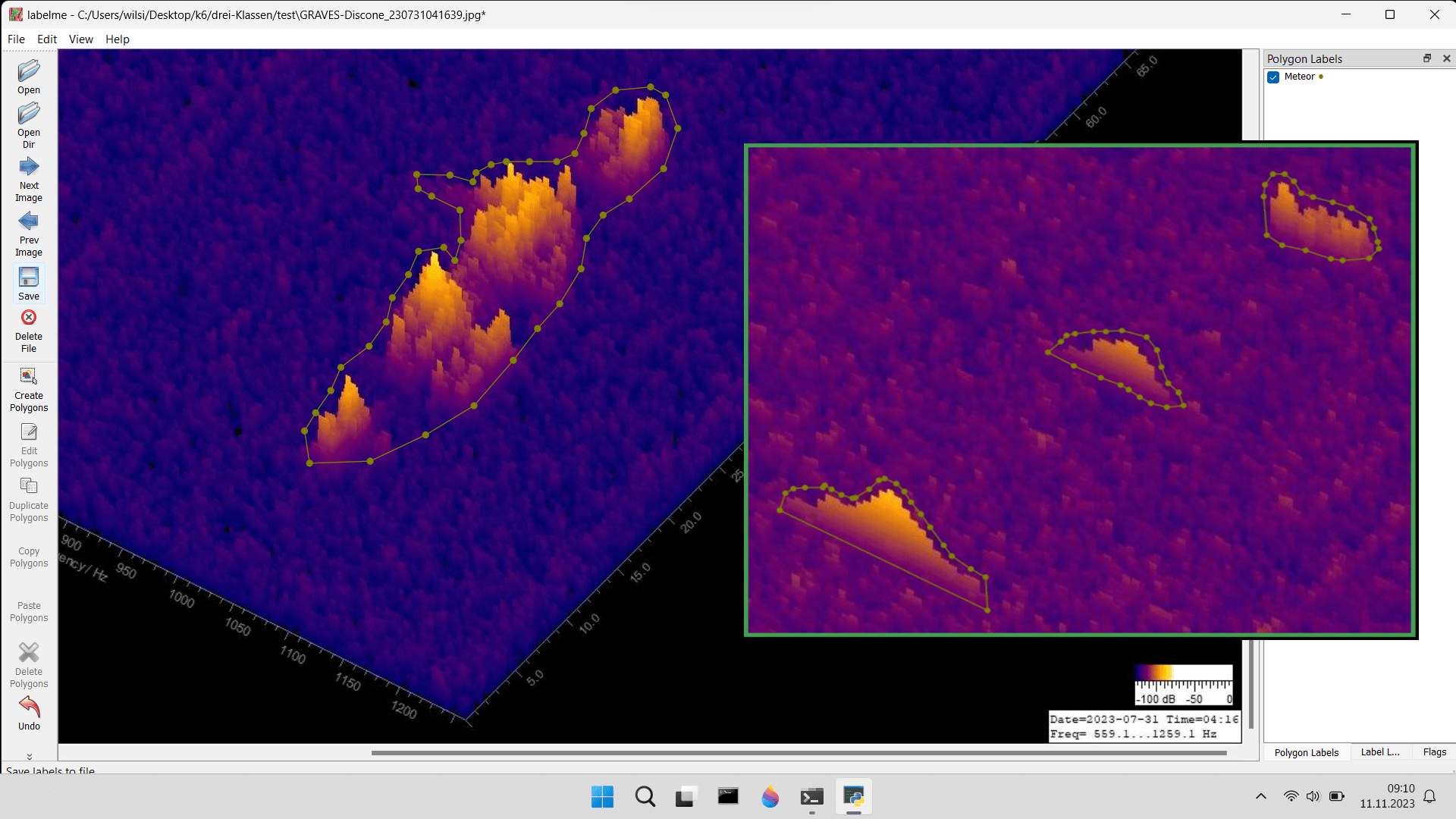
Figure 1 – Screenshot of the Labelme program. The inset shows that the three echoes can be labeled together in one plot. Different classes must not be labeled in one plot.
Labeling, i.e. creating the border and naming it with the class name, here Meteor, must be carried out for each signal. For demonstration purposes, an inset with three echoes was added to the screenshot. This is intended to show that the 600 plots contain significantly more than just 600 objects, perhaps three or four times as many. The boundary strip around the fragments of the large echo created by the switching process of the GRAVES antennas indicates the algorithm that such or similar echoes must later be viewed as a single meteor, as we see it as observers. The label data generated for each plot are then saved in a .JSON file. Finally, the files are divided into two folders: One third of each class is copied into a folder called TEST, two thirds are copied into the TRAIN folder. This so-called test-train split is used so that the algorithm can check its training with data that are not used in training. The key word for this is backpropagation.
A few details about the actual training and the calculation times can be found in the Benchtest chapter.
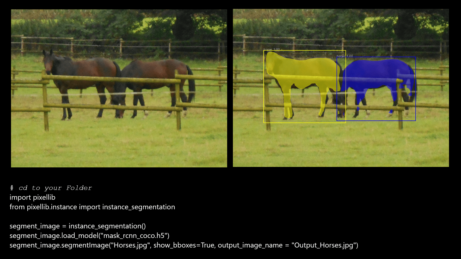
Figure 2 – Two horses are detected using the mask_rcnn_coco network. Only a very short code is required. (The photo was taken by the author.) Source: https://pixellib.readthedocs.io/en/latest/Image_instance.html
Figure 2 illustrates how divided / interrupted objects are treated: The mask_rcnn_coco network is used to analyze two horses that are divided by the picket fence. Of course, the horses are detected as a whole, just as we perceive it. Figure 2 also shows the short code used to examine the image.
How well the detection of a soft and fragmented meteor works is shown in Figure 3. The following short code would detect the echo in Figure 3:
import pixellib
from pixellib.instance import custom_segmentation
segment_image = custom_segmentation()
segment_image.inferConfig(num_classes= 3, class_names= [“BG”, “Artificial-Star”, “Background”, “Meteor”])
segment_image.load_model(“mask_rcnn_model.075-0.393305.h5”)
segment_image.segmentImage(“Meteor.jpg”, show_bboxes=True, output_image_name=”Output_Meteor.jpg”)
In this Python script the three new classes Artificial-Star, Background and Meteor and the self-created neural network mask_rcnn_model.075-0.393305.h5 are used.
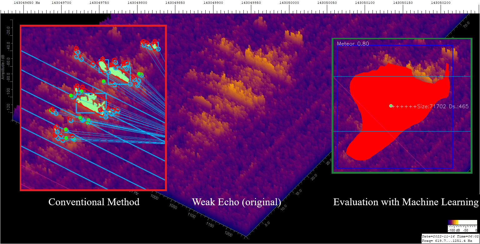
Figure 3 – The image shows the detection of a very soft echo using the conventional method compared to the machine learning method. The conventional method would log many echoes. I would have had to edit such an echo by hand. Further weak echoes that were correctly detected using the AI method are shown in the appendix Figure A13.
Arificial Stars
Starlink satellites are launched into space at short intervals, so that they increasingly appear in the GRAVES radar. Therefore, a separate class called Artificial-Stars was created. Meteors and satellites can be distinguished very well with ML because the metal surface produces a comb-like structure of the echo, see Figure 4.
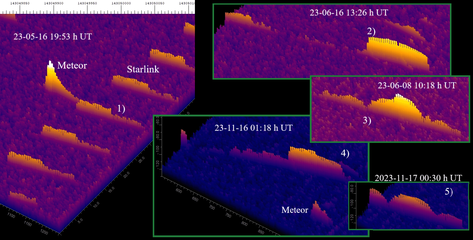
Figure 4 – A meteor and some Starlink satellites are shown on the left side of the image. The steps on the echoes (marked with 1) result from the change in direction of the transmission lobes. Furthermore, 4 echoes are shown on the right in the remaining figures, which presumably come from larger spaceships, see text.
The Starlink satellites basically provide an echo with a straight surface/envelope. The stage on the right of the echoes (labeled with 1) is generated by the switching process of the GRAVES antennas. The remaining satellite echoes (2 – 5) show a more or less curved envelope, indicating a more complex surface.
The image from the Starlink satellites (left in the picture) shows them shortly after release at an altitude of approximately 200 km, see also Figure 5. This would explain the small difference in size compared to the other objects if they were space stations. The ISS, for example, flies at an altitude of 400 km.
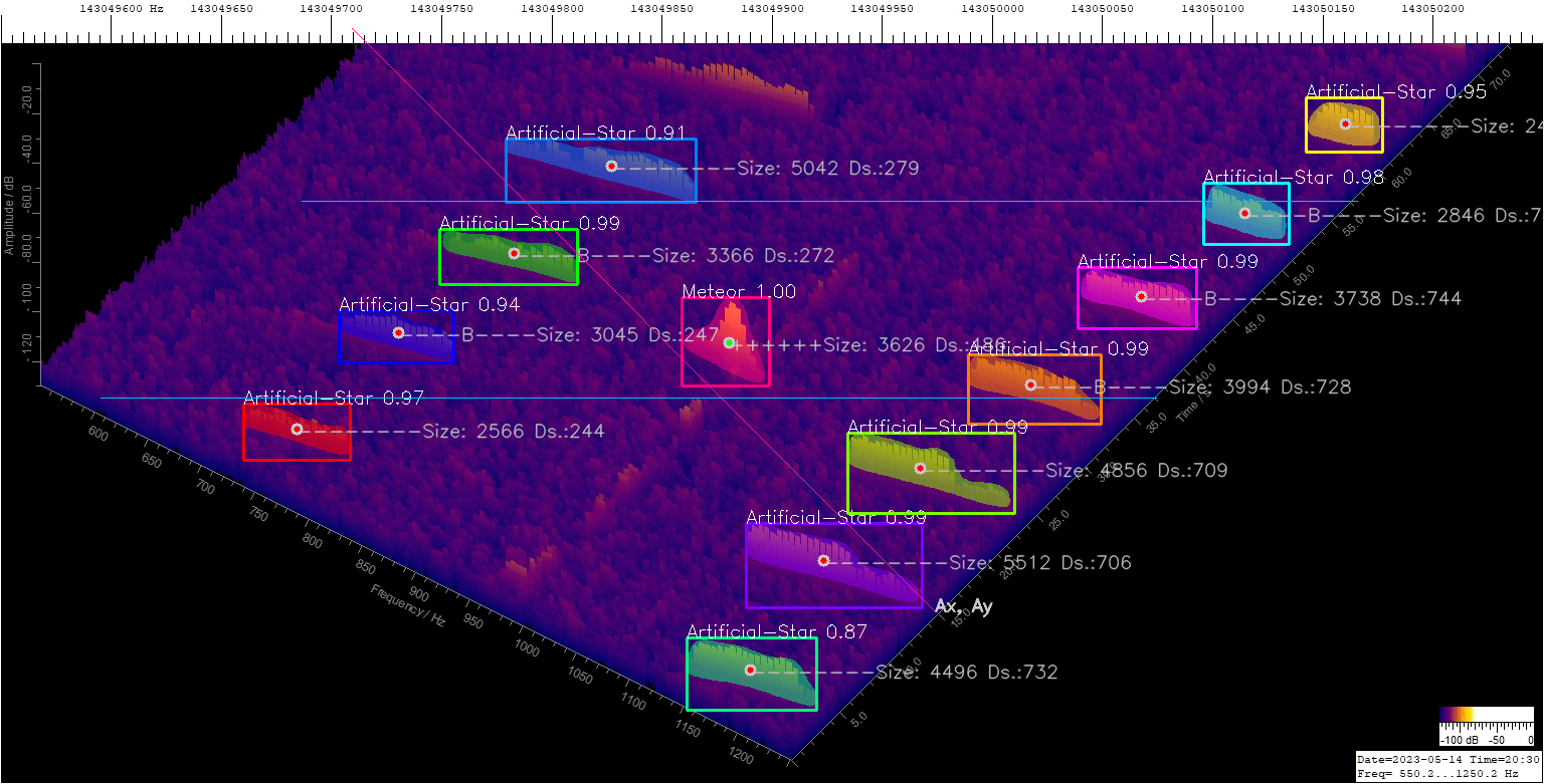
Figure 5 – A meteor in the middle of Starlink satellites was detected using ML. The echoes on the right and left belong to the same satellite. However, due to the switching process of the GRAVES antennas, they are not always exposed. One meteor and five satellites are logged. In this case, that’s two too many. However, such accumulations are rare.
Background
A separate class was created to detect interferences. Various crackling impulses and a disturbance carrier are labeled. In an early version I had also labeled the stripes/carriers that are caused by switching power supplies in LED bulbs etc, see Figure 6. However, not all types of interference need to be explicitly labeled. By training with images that contain both labeled echoes and unlabeled noise / interference, the model learns that these signals do not belong to the echo. Of course, prior knowledge is also incorporated through transfer learning. The model already knows the recurring frame or label. With the conventional method, everything had to be masked away.
Figure 6 shows that the ML detects the meteor even in presence of strong interference.
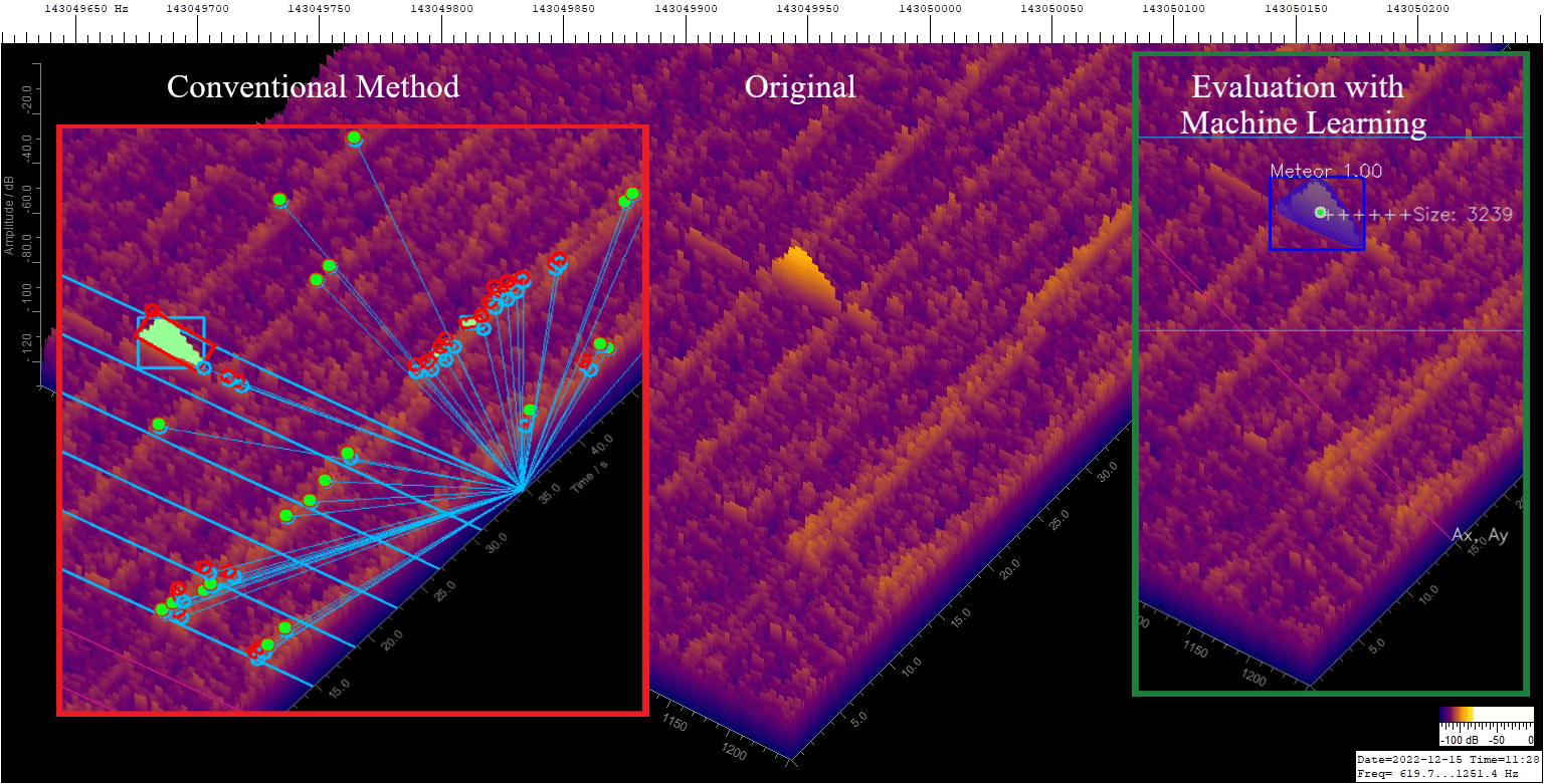
Figure 6 – The ML method can detect the meteor even in presence of strong interferences. With the conventional method, the disturbances trigger many hits and evaluation was no longer possible. With the ML method, evaluation is no problem. Another image (Figure A14) with a very small meteor s shown in the appendix.
4 The Evaluation
The evaluation software reads all the images addressed by file names and wildcards one after the other, usually those from an entire day. The total recording time per chart is approximately one minute. However, since the plots are saved every 20 seconds, only the contents of a 20-second time window need to be logged. Due to the long recording time, even large echoes that last significantly longer than 20 seconds are still recorded correctly. This is explained in Figure 7.
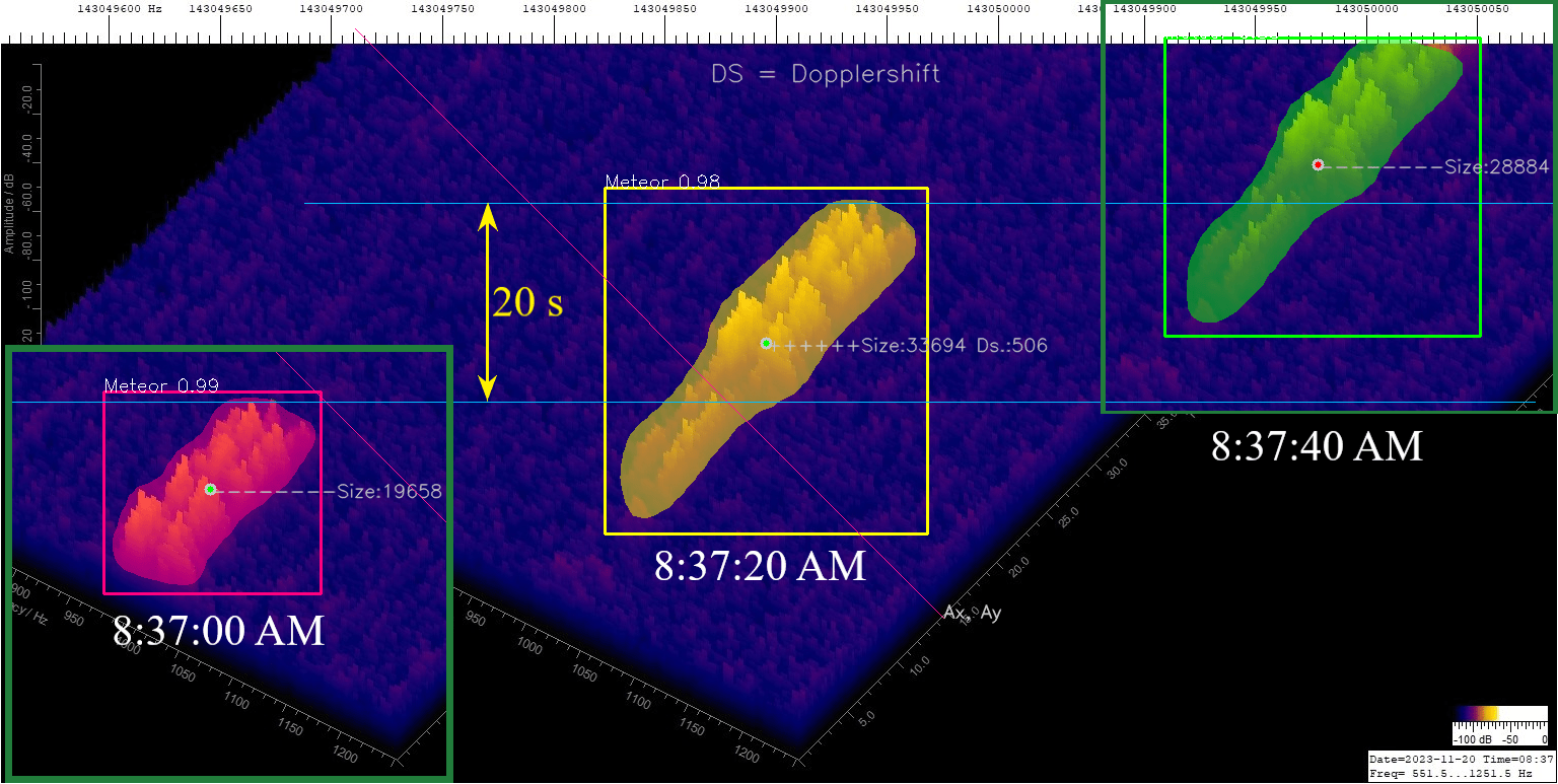
Figure 7 – Logging an Echo. Only the echo from 8:37:20 AM (yellow) is logged because the center of gravity is in the 20 s evaluation window. Figure A15 in the appendix shows an example of another large and soft echo being logged.
Figure 7 is based on a plot from 8:37:20 AM. Two insets, one on the left from 8:37:00 AM and one from 8:37:40 AM on the right edge, were added. So three recordings are displayed approximately 20 seconds apart. At 8:37:00 AM the meteor is partially at the bottom of the image but is not recorded because the center of mass is still below the blue line. At 8:37:20 AM the center of gravity is in the 20-second evaluation window and logging takes place. At 8:37:40 AM the center of gravity is again outside the evaluation area.
The Pixellib routines shown above then return information about the detected objects to the evaluation program. These are the classes, polygons of the areas, the probabilities and the boxes. The result can be displayed in debug mode. An example is shown in Figure 8.
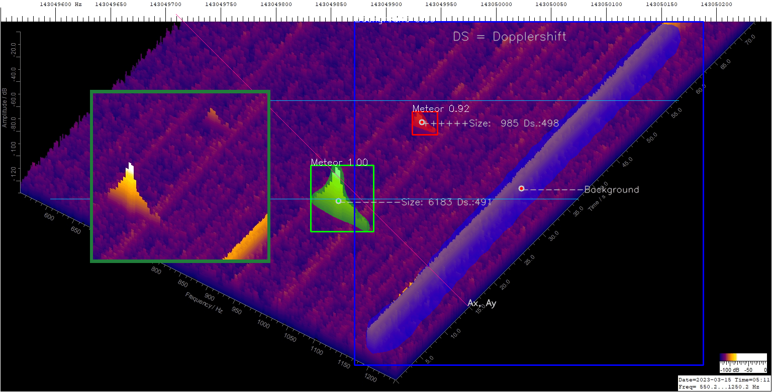
Figure 8 – Detection of two small meteors and a disturbance. In this diagram, only the small upper (red) echo is recorded because it lies between the two horizontal blue lines, i.e. in the 20 second window. The lower echo is in the evaluation window with the next plot. The inset on the left shows the original echoes.
Figure 8 contains two echoes and a disturbance that occurs occasionally and fortunately only on the right edge. I chose this plot to show that such disorders can be reliably detected. The upper small echo is below the level of the interference signal.
This type of AI/ML-investigation is called instance segmentation because multiple instances (meteors) are distinguished in one class. In the case of Figure 8, only the upper small meteor is recorded. The evaluation software determines the area and a relative Doppler shift is calculated from the center of gravity of the surface. The lower meteor is in the evaluation window with the next plot. After all plots have been examined, an overview is created, see Figure 9.
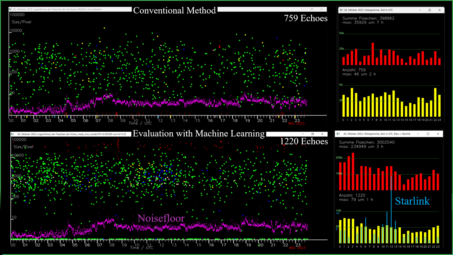
Figure 9 – Measured meteor sizes as a function of time, recorded on 26th October 2023. Each green dot represents an echo. The diagram in the lower half of the image shows that 1220 echoes were recorded using the AI/ML method. The blue dots and the blue histogram represent the Starlink satellites. The red dots are the logged interferences. For comparison, the evaluation using the conventional method is also shown in the upper diagram. Only 759 echoes are logged here, see text. The noise floor is determined by integrating a small area of background.
The points in the lower illustration in Figure 9 represent the measured echo sizes as a function of time for October 26, 2023 as an example. Around five orders of magnitude of the echo sizes are resolved. 1220 echoes were counted. The yellow histograms show the rate and the red histograms show the rate weighted by the size of the meteor echoes. The blue dots and blue lines represent the Starlink satellites.
To the Threshold
Figure 9 shows the evaluation using the conventional method for comparison purposes too. Significantly more echoes are detected with the ML method. The reason for this will now be examined using Figure 10. Two echoes are detected using the conventional method. The third middle echo is below the threshold. With the ML method, all three echoes are detected because there is no threshold. The absence of the threshold also means that the echoes are larger by a factor of 10 according to the ML method. (There are 10 times more pixels in the polygon.) The reason for this is that the conventional method only detects the peaks of the echoes that are above the threshold. The ML method also detects the part of the echo that lies in the background or noise. This is one of the big advantages of object detection with ML.
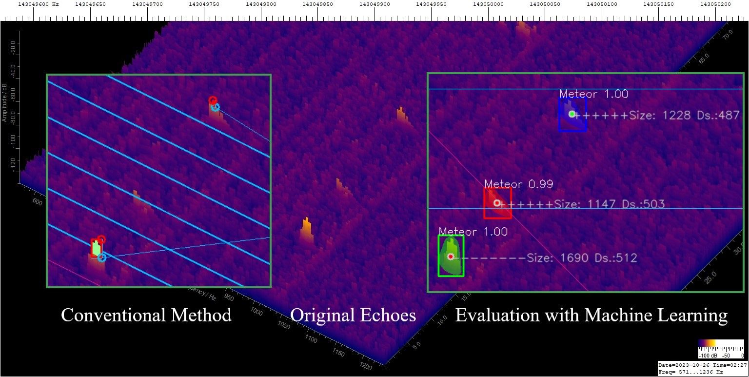
Figure 10 – With the conventional method, the threshold must be high enough so that disturbances do not trigger the recording. The ML method also detects weak signals.
5 Summary and Outlook
The so-called AI, or rather ML, is not a fad or something mystical, but a tool that can deliver very good results. I am particularly interested in the very small echoes in order to further investigate the In-Line-Peak, see Figure 11, the red dot. I would also like to investigate particle sorting in streams based on the Poynting-Robertson effect. To do this, small echoes in particular must be detected. The method shown here should help. Because of the interference in my residential area, I will test a new location in the future. It is the clubhouse of the chapter N62 Wüllen of the German Amateur Radio Club, see Figure 12. But at the moment it’s too cold and too dark, so realistically collecting data probably won’t really start until the Perseids in summer.
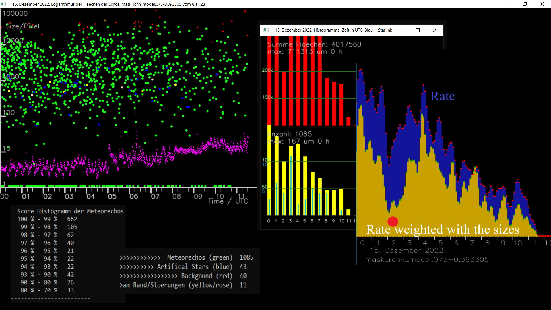
Figure 11 – Recording from December 15, 2022. I canceled the recording because of the interferences. An inset clearly shows the In-Line-Peak, see the red dot.
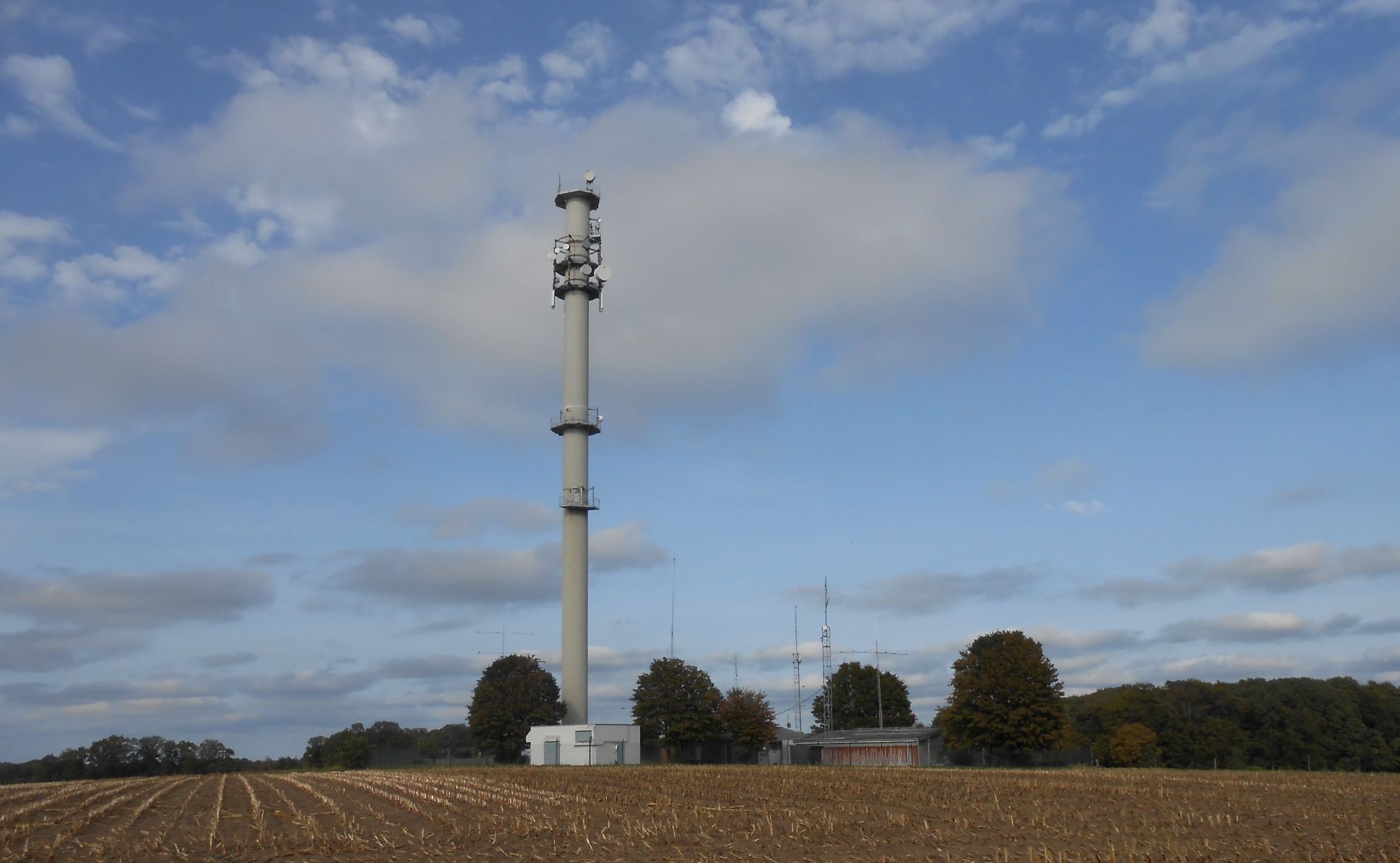
Figure 12 – Photo of the OV N62 clubhouse. It is a former NATO radio tower. (The photo was taken by the author.)
The project is constantly being developed. I would be happy to pass on the programs, the label data used and the model if anyone would like to participate.
Acknowledgment
Many thanks to Kerstin Sicking, Stefanie Lück and Richard Kacerek for proofreading the article. My special thanks go to Stefanie Lück for the many discussions in the Astronomie.de forum.
References
Sicking, W. (2022a). “A Notch in the Arietids Radio Data and a new so called In-Line-Effect”. EMetN, 7:5, 331-335.
Sicking, W. (2022b). “Radio observations on the Perseids and some other showers in August and September 2022”. EMetN, 7:6, 407-410.
Olafenwa, A. (2020). “PixelLib”. https://github.com/ayoolaolafenwa/PixelLib
He K., Gkioxari G., Dollár P., Girshick R. (2018). “Mask R-CNN”. Facebook AI Research (FAIR). https://arxiv.org/abs/1703.06870
Appendix
(Installation, a benchtest and a few additional images)
Installation
The important packages are Python3, Pixellib and the CUDA software for the RTX-3060 GPU.
Since Pixellib hasn’t been maintained for two years, installing it is a bit tricky, especially on Windows 11.
First you have to install Python 3.9.7 with appropriate dependencies.
Tensorflow 2.5 is the highest working version with Pixellib.
Tensorflow 2.5 installs an older version of Numpy with a module (scikit-image) that is not compatible in the current version. Another problem under Windows 11 is a bug in the labelme2coco program. It works with the very first version.
These versions and this sequence work on Windows 11 for the author:
pip3 install scikit-image==0.18.3
pip3 install numpy==1.19.5
pip3 install tensorflow==2.5.0
pip3 install imgaug……(it is 0.4.0)
pip3 install pixellib –upgrade
pip3 install labelme2coco==0.1.0
This is how you can view the installed versions:
C:\Users\wilsi>python
Python 3.9.7 (tags/v3.9.7:1016ef3, Aug 30 2021, 8:19:38 p.m.) [MSC v.1929 64 bit (AMD64)] on win32 Type “help”, “copyright”, “credits” or “license” for more information.
>>>import numpy
>>>print (numpy.__version__)
1.19.5
>>>
An exception is scikit-image. You import it with:
>>> import skimage
>>> print (skimage.__version__)
0.18.3
>>>
The installation ran with the default settings on the Windows 10 gaming PC.
If you want to install CUDA code for Nvidia GPUs, you need to know the compute capability of the GPU. My graphics card, the GeForce 3060 laptop GPU, has a compute capability of 8.6. Therefore, cuDNN 8.6 for CUDA 11.2 and the Cuda Toolkit 11.2 were installed.
Tensorflow then calculates in parallel.
Bench test
comparing the gaming PC with the Nvidia 3060 GPU and a normal i5 PC.
A short script from the tutorial is used for training: https://pixellib.readthedocs.io/en/latest/custom_train.html
I calculated 200 epochs to train the current model. I didn’t remember the total computing time, but the last saved epoch was epoch 92. It took an hour and 20 minutes up to that point on the gaming PC. An epoch therefore lasts just under a minute.
However, the model from epoch 92 was not used for the analyzes in this paper, but rather the model from epoch 75 (mask_rcnn_model.075-0.393305.h5) in order to prevent overfitting.
For comparison purposes, I calculated only one epoch on the i5 PC. It lasts 37 minutes. The 92 epochs of the gaming PC would therefore last 56.7 hours, i.e. 2 days and almost 9 hours. The i5 also works with its 4 cores in parallel: the load was up to 100%.
The analysis of the 4320 images from the 24 hours of October 26th, 2023 took 17 minutes on the gaming PC. To compare the analysis times, I only examined one hour of data on both computers: It takes 50 seconds on the gaming PC and 8 minutes on the normal PC, which would mean over 3 hours for data from a day. When analyzing, the GPU load of the gaming PC is in the range of 30%, while the GPU load during training is around 80%. The analysis does not benefit as much from the GPU, as images constantly have to be loaded.
This comparison should show that it is difficult to do machine learning without a GPU. It’s not just a one-off 2 days and 8 hours, but a lot of tests are necessary. I often see where the journey is going after 3-4 epochs. That’s a few minutes of computing time. On the PC it would then be 2 hours.
Supporting Images
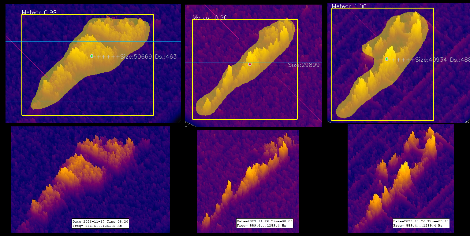
Figure A13 – Further weak echoes that were correctly detected using the AI method.
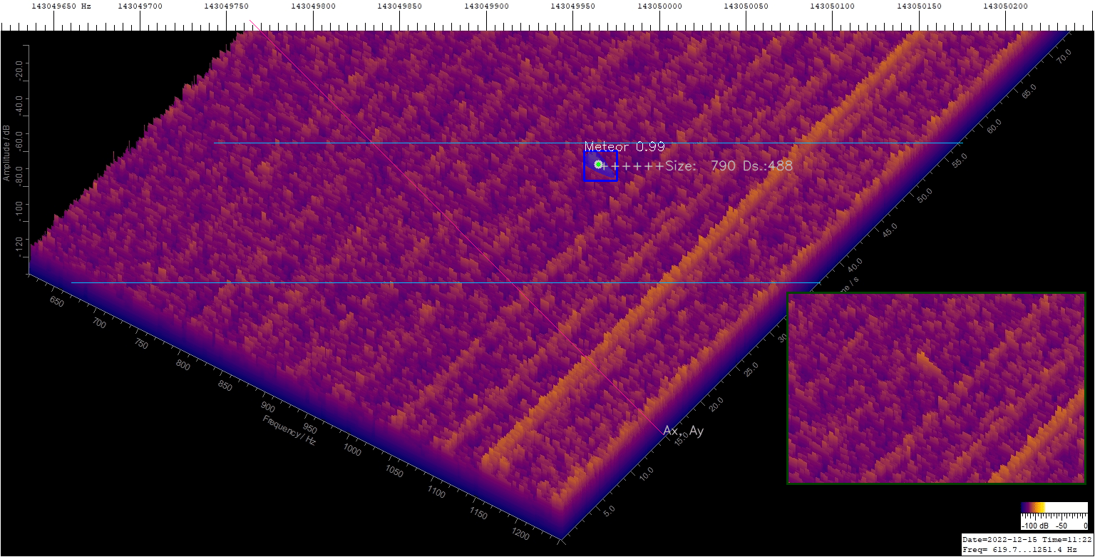
Figure A14 – The ML method can detect the very small meteor even in presence of strong interferences.
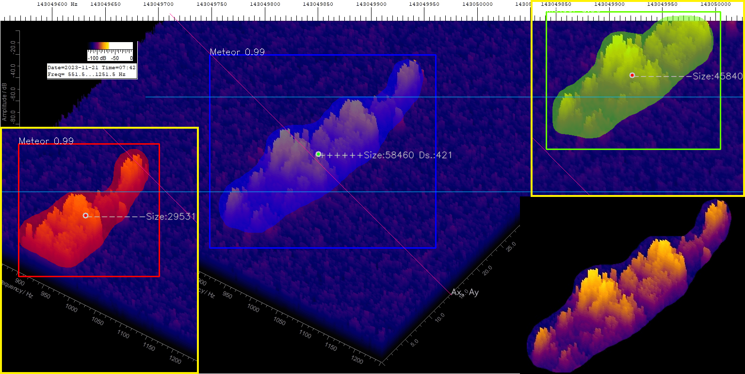
Figure A15 – The picture shows how a soft echo that lasts significantly longer than 20 s is logged correctly. The ++++ show that it was logged.
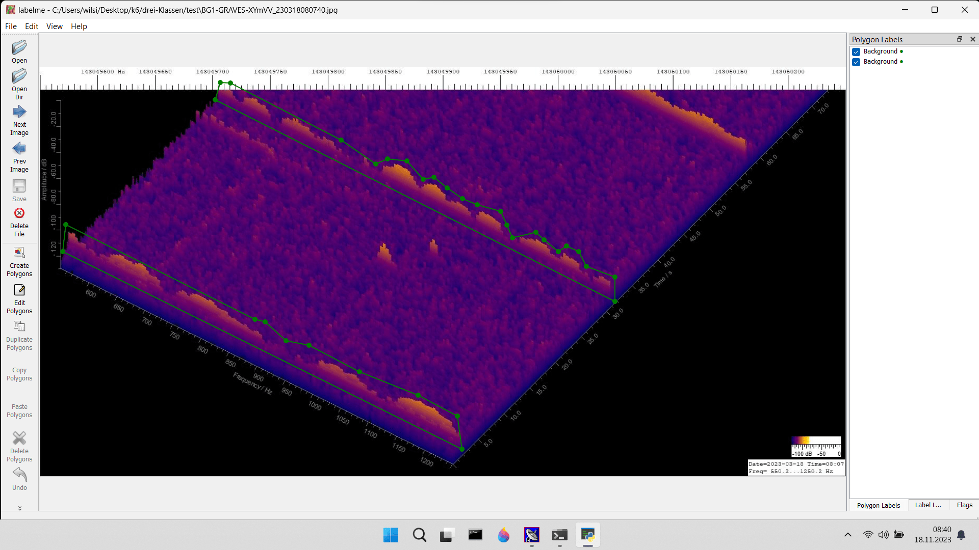
Figure A16 – An example of disturbances/clicking impulses is shown in a Labelme screenshot.
End of File
WiSi 28.11.2023


I find the work of Wlihelm Sicking interesting and would like to discuss his approaches and compare to my own. I do not have his contact details (email). My email given below may be passed to him.
Hi Mike.
Thank you for your interest.
I sent you an email.
Best regards
Wilhelm