Abstract: The Global Meteor Network consists of over 450 video cameras in 30 countries. Most of these cameras are part of various regional networks. A significant challenge is to optimally orient the cameras within a regional network to maximize the volume of atmosphere that is observed by at least two cameras. We demonstrate the use of an integer linear programming approach to optimize camera coverage for the New Mexico Meteor Array.
1 Introduction
The Global Meteor Network consists of over 450 video cameras in 30 countries that are observing and measuring meteor activity on a nightly basis (Vida et al., 2021). Achieving valid meteor trajectories requires that meteors be observed by at least two cameras. A significant challenge is to optimally orient the individual cameras within a regional network of cameras so as to maximize the volume atmosphere that is within the field of view of least two cameras.
The Art Gallery Problem is a well-known problem in computational geometry. It addresses the problem of guarding an art gallery with the minimum number of guards who can keep every piece of art within the gallery under their constant gaze. It is a special case of the more general problem of maximizing surveillance of selected targets by a limited number of sensors. There is an extensive literature on this topic (Mavrinac and Chen, 2013). However, we found little in the literature that is directly applicable to the unique requirements associated with meteor monitoring. Here, the challenge is not to keep a few selected targets always in view with the minimum number of sensors, but to find the largest volume of contiguous space that can be kept within the constant view of two or more cameras. Furthermore, because these cameras are operated by volunteer owners, it is generally not possible to optimally choose the location of the camera, nor is it always possible to use what might be the optimal azimuth and elevation angle due to obstruction by terrain, trees, buildings, utility poles, etc.
2 Approach
We employ the Target in Sector (TIS) approach to the problem of optimizing multi-camera coverage of multiple targets by a network of directional cameras as described by Sadik et al. (2015). This is commonly referred to as the k-coverage problem, where k refers to the number of cameras covering a target.
A target is deemed coverable by a camera if it is within the angular sector defined by the field of view of the camera and within the sensing range of the camera. Conducting TIS tests over every possible orientation of every camera for each target leads to a 3-dimensional coverage matrix of M targets and N cameras with P orientations where each binary element of the matrix is assigned a value of 1 when target Mm is covered by camera Nn at orientation Pp or, otherwise, the matrix element is assigned the value of zero.
For meteor detection, the targets are the gridpoints of a three-dimensional Cartesian grid that covers the altitude layer where meteors are typically observed above a geographical region of interest. While the magnitude of the horizontal dimensions is limited only by the computational power that it takes to numerically solve the optimization problem, we have generally limited the Cartesian grid to less than 1000 km × 1000 km at 10 km resolution. The vertical dimension of the grid is between 70 km and 120 km at 10 km resolution. This region is referred to as the Region of Optimization (RoO).
We define 24 possible orientations for each camera by designating 8 azimuths (N, NE, E, SE, S, SW, W, NW) and up to 3 user-selectable elevation angles for each elevation. The most common camera/lens arrangement in the GMN network uses the IMX291 camera fitted with a 3.6mm f/0.95 lens. This combination yields a nominal 88° × 48° field of view (Vida et al., 2021). It is also conveniently suitable for the computation of the binary coverage matrix via the TIS method described above.
The effective sensing range of the cameras was estimated from an analysis of over 45000 meteor observations made by all 23 stations in the New Mexico Meteor Array (NMMA) during December 2020. Analysis of those observations revealed that 99% of meteors detected were within 320 km of the stations detecting them.
The software that processes the meteor observations detected by the cameras, RMS, also calculates a polygon representing the field of view at 100 km altitude from the stellar astrometric calibration data that accounts for lens distortion and asymmetry. In a similar way, the field of view can also be visualized by plotting the projected location of meteor observations in the horizontal plane at 100 km altitude from the azimuth and altitude of the observations. In Figure 1, the blue polygon represents the RMS-calculated field of view at 100 km and the grey markers are the projected locations of 7238 meteor observations (made in December 2020) at 100 km for one camera in the network, US000J. Several features are apparent. Because meteors exhibit a wide range of magnitudes, the density of observations decreases with increasing distance from the station due to atmospheric scattering and extinction of light from the fainter meteors. Some (4.4%) observations fall outside of the polygon. The reason for this is not clear. The asymmetry of both the polygon and the distribution of observations may be the result of lens asymmetry or because the camera is not perfectly level.
Figure 1 also shows (in yellow) the nominal 88° × 48° field of view as computed by the TIS test as described above. This field of view encompasses 71.9% of the observations. We found that increasing the horizontal width to 96° was a better match to the width of the RMS-polygon. We decreased the vertical height of the field of view from 48° to 46° because all the platepar files we examined from the cameras in the Lowell and NMMA networks reported a vertical field of view of 46°. The resulting field of view of 96° × 46° at 100 km and limited to a range of 320 km as computed by the TIS test is shown in green in Figure 1. This field of view encompasses 74.2% of the observations and is used for all of the results presented below.
Many camera owners rely on the 3DFOV tool provided on the GMN website to aid pointing of cameras. Figure 1 shows that field of view in red. Note that 64% percent of the meteor observations are within that trapezoidal polygon.
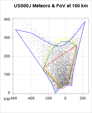
Figure 1 – Meteors detected at 100 km by US000J and representations of the field of view: RMS (blue), FOV3D (red), 88° × 48° sector (yellow), 96° × 46° sector (green). See text for details.
After the binary coverage matrix has been created by the TIS test, the next step is to formulate an objective function that can be numerically solved using integer linear programming techniques.
The objective function is the function to be maximized by the numerical solver. Although a meteor trajectory and orbit can be calculated with a minimum of two observations from two stations, it is desirable to have at least three camera coverage for a more robust solution. Therefore, the objective function maximizes the number of targets covered by three or more cameras (k ≥ 3).
Implementation of the model is performed with SAS® software (The output for this paper was generated using SAS software. Copyright © 2021 SAS Institute Inc. SAS and all other SAS Institute Inc. product or service names are registered trademarks or trademarks of SAS Institute Inc., Cary, NC, USA. ). Specifically, SAS software generates the binary coverage matrix. The SAS OPTMODEL Procedure implements a mixed integer linear programming solver that finds the optimal orientation of each camera that maximizes the objective function. SAS software is also used to analyze and display the results. SAS software is a cloud-based service freely available through SAS OnDemand for Academics.
Figures of Merit
An important use of the model is to explore of how the addition of new or hypothetical cameras or relocation or re-aiming of existing cameras might affect the overall coverage. A key question is how to measure the quality of one proposed solution versus another. There are several ways to evaluate a solution.
The simplest metric is the Objective Value. This is the value of the function being maximized by the model. It is simply the number of gridpoints covered by 3 or more cameras (k ≥ 3).
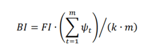
Sadik et al. (2015) proposed what they call a Balancing Index. It combines the concept of a Fairness Index that measures the uniformity or fairness of coverage with an additional metric that measures the extent to which the desired goal of 3-camera coverage has been met. Mathematically, the Fairness Index is expressed as:
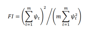
where m is the number of targets, and ψt is the number of times target t is covered. Note that ψt is restricted to less than or equal to k to avoid biasing the result by targets with > k camera coverage. Sadik et al. (2015) recognized that this metric is imperfect because it favors solutions that yield uniform coverage.
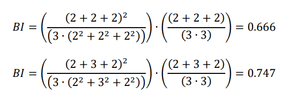
Consider a simple case (adapted from Sadik et al. (2015)) with only 3 targets and where 3 camera coverage (k = 3) of each target is desired. A solution where each target is covered twice (2, 2, 2) is fairer than a solution where two targets are covered twice and one target covered three times (2, 3, 2). The Fairness Index FI for both solutions is given below:
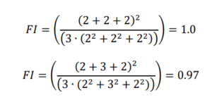
The (2, 2, 2) solution, while fairer than the (2, 3, 2) solution, fails to achieve the desired 3-camera coverage for any of the targets. Sadik et al. (2015) modify the concept of the Fairness Index by introducing a term that measures the achieved coverage as a fraction of the maximum possible coverage. Mathematically, the Balancing Index is given by:
where km is the product of the desired optimal coverage (k = 3) and the total number of targets m.
Using the example from above, the Balancing Index for the two solutions is:
The Balancing Index favors the (2, 3, 2) solution and is a more useful metric for evaluating possible solutions. Note that this metric, like the Objective Value, is based on the number of gridpoints covered and the number of times each gridpoint is covered.
In meteor science the quality of the coverage is as important, if not more so, as the extent of the coverage. Quality of coverage can be measured by the convergence angle. From geometry, on a 3-dimensional grid, a plane can be defined by a line and a point. The convergence angle, Qc, is defined as the angle between two planes where each plane is defined by the linear track of the meteor and the location of each of two stations. A meteor trajectory obtained from a pair of observations by two stations with a high convergence angle is, all else being equal, superior to a solution from a pair of observations with a low convergence angle.
From the model output, we identify the subsets of gridpoints within the Region of Optimization that are within the joint field of view of every unique combination of cameras. For each subset, 100 random meteors (Random meteors are generated between start altitudes of 90–120 km and end altitudes of 70–100 km while ensuring that the start altitude is higher than the end altitude. The track is at least 10 km in length and the entry angle is between 15 and 90 degrees.) are generated within the bounds of that region. The mean convergence angle among the cameras that hold that region within their joint field of view is calculated. If a region is within the view of only two cameras, then the Qc Score for the region is calculated as the mean of the convergence angle for the 100 meteors weighted by the number of gridpoints within that region. If three or more cameras cover the region, then for each of the 100 random meteors we identify the camera pair with the maximum Qc value. The Qc Score for that region is defined as the mean of the maximum Qc values for the 100 meteors weighted by the number of gridpoints within the region. The final Qc Score for the entire Region of Optimization is then taken as the mean of the Qc Score for all sub-regions. Note that the Qc Score is a relative measure that can only be used for evaluating the coverage of one possible arrangement of cameras vs other possible arrangements within a given RoO.
3 Results
Two-station network
The simplest of networks consists of two cameras. This is the minimum number of cameras necessary to compute a meteor trajectory and orbit. For eight possible azimuths, there are four possible camera orientations (Figure 2). The optimal choice depends on the elevation angle of the cameras and the distance between the stations. The optimal elevation angle is the lowest angle that has a clear view of the sky for both cameras. The optimization model was used to determine the optimal orientation as a function of the distance between the stations. Table 1 shows the recommended orientation as a function of the elevation angle and the distance between the stations.
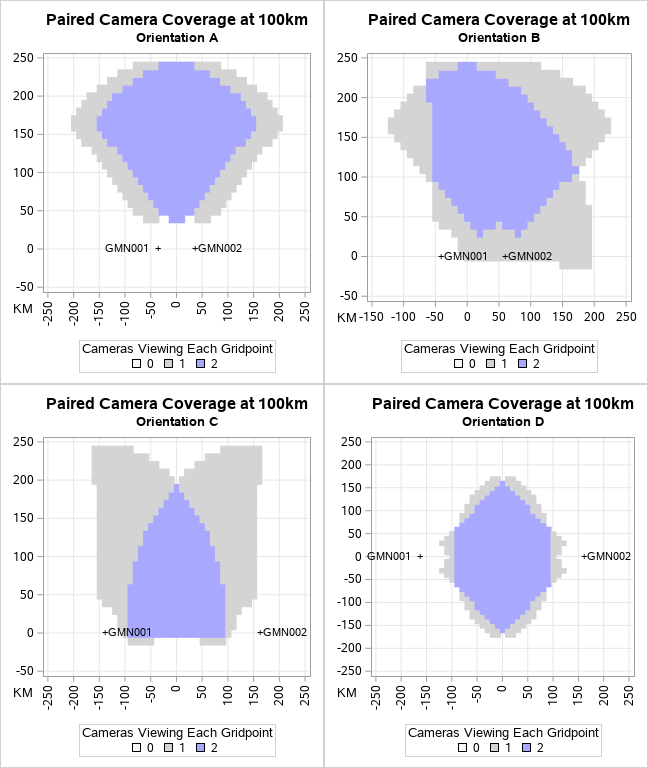
Figure 2 – Four possible camera orientations for a two-station network. For Orientation A, GMN001 & GMN002 are both aimed perpendicular to the line between the two stations. For Orientation B, GMN001 is oriented perpendicular to the line whereas GMN002 is at a 45° angle toward GMN001. For Orientation C, each camera is oriented at a 45° angle towards each other. For Orientation D, the two cameras are aimed toward each other.
Table 1 – Two-camera orientation as function of elevation angle and distance between hypothetical stations GMN001 and GMN002. See Figure 2 for a description of orientations A through D.
| Elevation Angle | ||||
| Orientation | 35 ° | 40 ° | 45 ° | 50 ° |
| A | <100 km | <80 km | <70 km | <60 km |
| B | 100-190 km | 80-180 km | 70-135 km | 60-110 km |
| C | 190-320 km | 180-290 km | 135-270 km | 110-200 km |
| D | >320 km | >290 km | >270 km | >200 km |
Small Network
A more complex challenge was to optimize the pointing of a small network of three stations located in Southern California. Initially, each station hosted a single camera. In 2021, the Lowell Observatory began installing and activating a network of cameras throughout Arizona. The field of view of some of these cameras extends westward into Southern California. Figure 3 shows the initial state of the coverage of the Lowell network and the three stations in Southern California at an altitude of 100 km.
Two of the three California stations were in the process of being upgraded with the addition of a second camera. So, the challenge became to optimize the pointing of five cameras at three locations so as to maximize the intersection with the field of view of the Lowell cameras. The fields of view of the Lowell cameras were treated as fixed and the Southern California cameras were optimized to maximize the volume of atmosphere covered by at least three cameras from both networks.
The first optimization calculations produced a result where both cameras co-located at a single location were oriented on the same azimuth and elevation. Although this produces two observations of a meteor by two cameras, there is no separation between the cameras. The convergence angle is zero and no trajectory solution is possible.
In these cases, the co-located cameras were treated within the optimization model as a single “virtual camera” with a horizontal field of view that is twice the width of a single camera. The model solves the optimization problem for the virtual camera. The physical cameras are aimed so that the boundaries of their respective fields of view overlap slightly at the azimuth recommended by the model for the virtual camera. Figure 4 shows the optimized coverage. The blue box shows the region where coverage is optimized by the model. Stations designated with the prefix VS are virtual stations with two co-located physical cameras. VS0S1R is a composite of physical cameras US000S and US001R. Whereas VS0V1Q is a composite of physical cameras US000V and US001Q. In this case, the optimal result was for US001E, VS0S1R and VS0V1Q to all be aimed at the 135° azimuth at 35° elevation. For the virtual station VS0S1R, the two physical cameras (US000S and US001R) were pointed at 180° and 90° respectively. The same holds true for virtual station VS0V1Q where the two physical cameras US000V and US001Q were also pointed at azimuths of 180° and 90°. The improvement in coverage is clearly evident in Figure 4. The figures of merit as represented by the Objective Value, Balancing Index and Qc Score as shown in Table 2 provide a more quantitative way to comparatively judge coverage pre- and post-optimization.
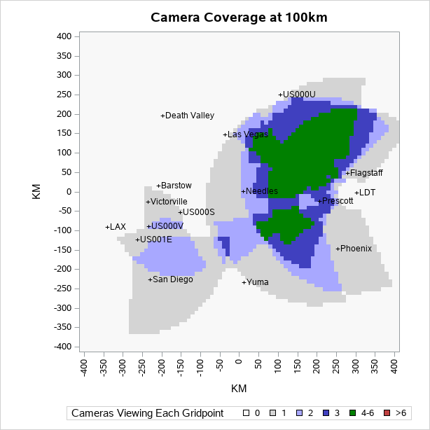
Figure 3 – Coverage at 100 km by the Southern California network and Lowell network before optimization.
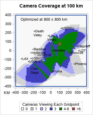
Figure 4 – Coverage at 100 km by the Southern California network and Lowell network after optimization.
While in this instance it’s clear from inspection of Figure 4 that the coverage after optimization is a dramatic improvement, it may not always be so clear.
Consider the hypothetical possibility that US001E could alternatively be located in Victorville, CA. It would be useful to know how this would affect network coverage. We ran the model for this configuration and found that the recommended camera orientations would be unchanged. But the entry for “Victorville option” in Table 2 shows that all the figure of merit scores are lower. Locating the camera in Victorville would not be an improvement over the current location.
The cameras of this network were re-aimed and re-calibrated in the summer of 2021 and are now aligned and operating as indicated in Figure 4.
Table 2 – Figures of merit for region of optimization.
| Figure of Merit | Pre-Optimization | Post-Optimization | Victorville option |
| Objective Value | 4592 | 10048 | 9620 |
| Balancing Index | 0.044 | 0.100 | 0.098 |
| Qc Score | 55 | 71 | 65 |
Large Network
Building on the success of the Southern California network, we moved to a similar problem but on a larger scale with the 23 cameras that comprise the New Mexico Meteor Array (NMMA). Here, too, the goal was to optimize the pointing of the NMMA cameras to maximize intersection with the cameras of the Lowell network whose fields of view extend eastward into New Mexico. In addition, a goal of the NMMA is to maximize coverage over the state of New Mexico.
Figure 5 shows the coverage at 100 km for the cameras in the Lowell network in eastern Arizona and extending into western New Mexico. Figure 6 shows the combined coverage at 100 km of the NMMA, as currently configured, with the Lowell network. The current coverage evolved prior to the establishment of the Lowell network. It was originally designed with the primary goal of maximizing coverage over the Albuquerque metropolitan area. The blue box is a 540 km by 700 km area that indicates the region designated for optimization. It covers most of the state of New Mexico and a bit beyond. It overlaps the outer limits of coverage from the Lowell network where there is less than 3-camera coverage.
As before, the orientation of the Lowell cameras was held constant while the orientation of the NMMA cameras were subject to optimization. If a given orientation of a camera results in an obstructed field of view, then that orientation becomes a forbidden orientation within the model. The three allowed elevation angles are 35, 45 and 55 degrees. Figure 7 show the coverage at 100 km after optimization. Table 3 gives the figures of merit for the Region of Optimization shown in Figures 6 and 7. Although the improvement is obvious from the figures, the increases in the figures of merit confirm the improvement. Work is presently underway to re-orient the NMMA cameras to their optimal orientations and establish the required new calibrations.
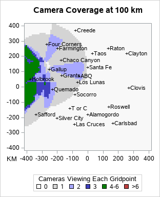
Figure 5 – Extension of coverage at 100 km by the Lowell Network into New Mexico.
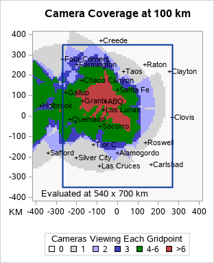
Figure 6 – Coverage at 100 km by the NMMA and the Lowell network before optimization.
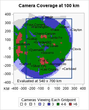
Figure 7 – Coverage at 100 km by the NMMA and the Lowell network after optimization.
Table 3 – Figures of merit for region of optimization.
| Figure of Merit | Pre-Optimization | Post-Optimization |
| Objective Value | 7406 | 18433 |
| Balancing Index | 0.35 | 0.78 |
| Qc Score | 11.9 | 25.6 |
4 Conclusion
The TIS approach of modeling the field of view of the cameras as a sector with a fixed range is conceptually simple, easy to implement, still useful for orienting cameras within a network, but not ideal. A different approach is needed to more accurately capture the complex shape and asymmetry of the actual field of view of the cameras. This could even be expanded to include the effects of atmospheric extinction and sensitivity loss. We are investigating an alternative approach that determines, for every possible camera orientation, which grid points are covered by the irregular polygon that represents the field of view.
The goal of the Global Meteor Network is: “No Meteor Unobserved”. One key to achieving that goal is optimal orientation of the cameras within the regional networks that comprise GMN. This work presents a methodology to optimize the orientation of multiple cameras so as to maximize the likelihood of simultaneous detection of meteors.
Acknowledgment
We thank the NMMA camera owner/operators without whom this work would not be possible: Peter Eschman (Coordinator), John Briggs, Ollie Eisman, Jim Fordice, Bob Greschke, Larry Groom, Tim Havens, Bob Hufnagel, Ron James Jr., Steve Kaufman, Jean-Baptiste Kikwaya, Bob Massey, Alex McConahay, Robert McCoy, Dave Robinson, Jim Seargeant, Eric Toops, Bill Wallace and Steve Welch.
We thank Denis Vida for his insights leading to the development of the Qc Score as a figure of merit.
References
Mavrinac A., Chen X. (2013). “Modeling coverage in camera networks: a survey”. International Journal of Computer Vision,101, 205–226.
Sadik M. M., Malek S. M. B., Rahman A. (2015). “On balanced k-coverage in visual sensor networks”. Journal of Network and Computer Applications, 72, 72–86.
Vida D., Šegon D., Gural P.S., Brown P. G., McIntyre M. J. M., Dijkema T. J., Pavletić L., Kukić P., Mazur M. J., Eschman P., Roggemans P., Merlak A., Zubrović D. (2021). “The Global Meteor Network – Methodology and First Results”. Monthly Notices of the Royal Astronomical Society, 506, 5046–5074.