By Paul Roggemans, Denis Vida, Damir Šegon and James M. Scott
Abstract: This article explains the procedure used by the Global Meteor Network to identify meteor showers using meteoroid orbits. Frequently used astronomical terms are explained for people unfamiliar with these terms. The practical application of this method is described with a case study on a newly discovered shower, M2025-Y1, which appears as an outburst caused by an unknown dust trail related to the parent body comet 12P/Pons-Brooks and the December kappa-Draconids.
1 Introduction
Although the first scientific meteor observations started in the early 19th century, meteor showers were known to radiate from a common point in the sky for many centuries. Ordinary people who witnessed meteor storms described it as if stars moved creating a tunnel effect. Major meteor showers were informally named according to the constellation from where the meteors seemed to radiate from, e.g. the Perseids from Perseus in August, the Leonids from Leo in November. This reminds us of the Quadrantids in January, which is from the obsolete constellation Quadrans Muralis defined by the French astronomer Jérôme Lalande in 1795. In 1922, this constellation was removed by the International Astronomical Union (IAU) when the official modern constellations were defined.
For major showers the identification can be done on sight during their maximum activity. However, there are many hundreds of dust trails crossing the Earth orbit which produce only weak activity hidden within the overall sporadic activity. Even major showers are hard to distinguish from sporadic activity when their number of meteors is statistically irrelevant before and after their maximum.
19th century astronomers developed visual observing techniques to plot meteors on star maps or on a star globe, tracing the trail seen at the sky backwards to reveal the radiant – the point in the night sky from where it was supposed to come. This backwards projection of meteor trails on star maps in gnomonic projection remained popular among amateur meteor observers in the 20th century. However, the presence of the sporadic background radiants and the effect of small-number statistics made it somewhat like gambling about the possible radiant association. More about the history and different meteor observing techniques can be found in the “Handbook for meteor observers” (Rendtel, 2020).
Meteors that belong to a meteor shower can be distinguished by their orbits since all particles within a meteoroid stream are spread along a common orbit (Figure 1). Since low light camera networks became affordable to the amateur community, large numbers of meteoroid orbit data have been collected. The properties determined for these meteoroid orbits offer a reliable alternative for meteor shower identifications.
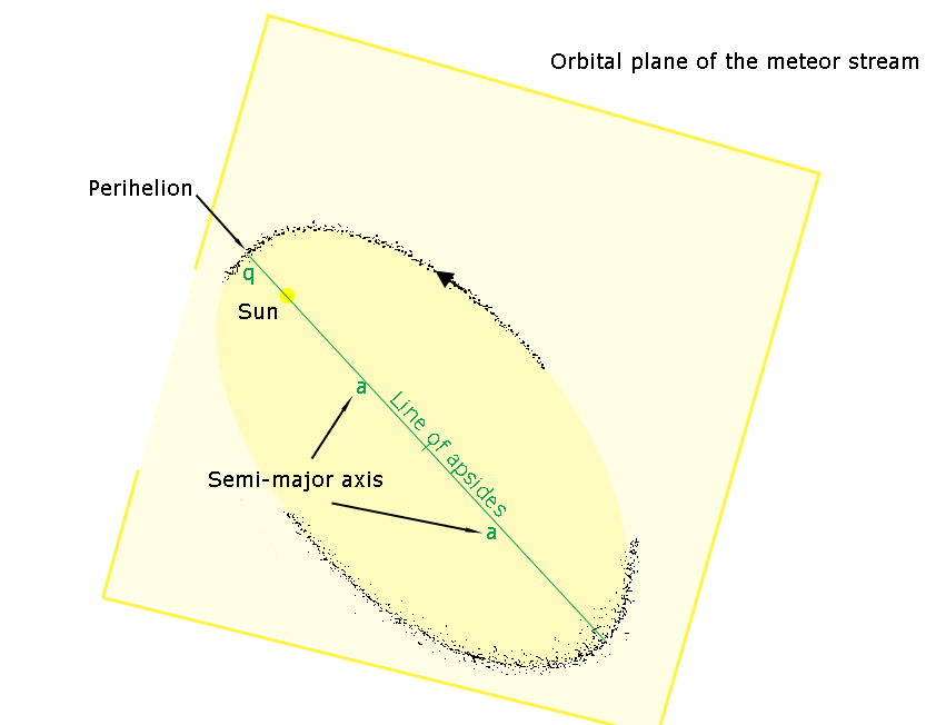
Figure 1 – Schematic presentation of a meteoroid stream with particles dispersed along an elliptic shaped orbit.
2 The orbital elements
For meteoroid orbits we use five parameters that describe the shape, size and orientation of the meteoroid orbit. These parameters are known as the Keplerian elements, with the semi-major axis a, eccentricity e, inclination i, longitude of the ascending node Ω and argument of periapsis (perihelion) ω. The orbital elements are basic geometry using references like the ecliptic plane and the vernal equinox (see Figure 2).
The shape of the meteoroid orbit is an ellipse with the Sun in one of its foci. The perihelion is the position where the orbit is at its smallest distance from the Sun. The aphelion is the position at the largest distance from the Sun. The perihelion distance q is the distance of the perihelion point to the Sun, expressed in Astronomical Units with 1 Astronomical Unit = the average distance between the Earth and the Sun.
Semi-major axis a is half the distance between the perihelion and the aphelion, expressed in Astronomical Units.
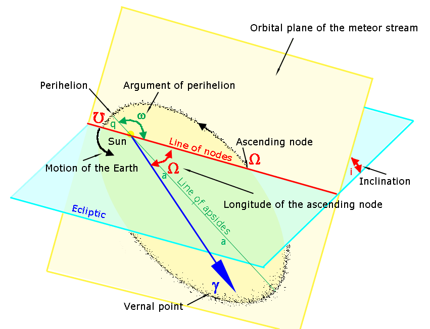
Figure 2 – Schematic presentation of a meteoroid stream with orbital elements in the ecliptic plane and the orbital plane of the meteoroid stream.
The other elements are measured in the ecliptic plane, which is the plane of the orbit of Earth around the Sun, and in the meteoroid orbit plane. The Vernal or Spring equinox is the position of the Earth where the Sun is crossing the Earth’s equator from South to North. The line of nodes is the intersection of the orbital plane of the meteoroid stream with the ecliptic plane.
The longitude of the ascending node Ω is the angle from the ascending node of the orbit to the direction of the Vernal equinox.
Argument of perihelion (periapsis) ω gives the orientation in the orbital plane, as the angle measured from the ascending node to the perihelion. The longitude of perihelion Π is defined as the sum of Ω and ω.
Inclination i is the vertical tilt of the orbital plane to the ecliptic, measured at the ascending node. Inclinations from 90° to 180° are called retrograde orbits.
The eccentricity e defines the shape of the ellipse. A perfect circle has e = 0, e < 1 is an ellipse, e > 1 is a hyperbolic orbit, and e = 1 is a parabola. Some simple equations allow to compute some of the orbital parameters based on a few known parameters, like the semi-major axis a derived from the perihelion distance q and eccentricity e, or the aphelion distance Q derived from semi-major axis a and eccentricity e: 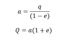
3 Ecliptic versus equatorial coordinates
In astronomy books, the positions of stars, nebula and other objects, including meteor shower radiants, are given in equatorial coordinates in Right Ascension and Declination with the Celestial Equator as reference plane. It is easy to find positions at the sky with a classic star atlas or to operate a telescope as these coordinates are aligned with the rotation of the Earth. To study objects like planets, minor bodies and meteoroid streams in our Solar System it is more convenient to use Ecliptic coordinates with the Ecliptic or Earth’s orbital plane as reference plane. The difference between the two coordinate systems is in the reference planes and their poles, tilted by about 23.5°. Equatorial coordinates can be converted into ecliptic coordinates by a simple coordinate transformation. More detailed information on coordinate transformation and celestial mechanics can be found in the work “Astronomical Algorithms” by Jean Meeus (1998), which is available for free download.
Instead of using calendar dates to define time we use the Solar Longitude, which is a measure of the position of the Earth in its orbit around the Sun, with the vernal equinox at Solar Longitude zero. The Solar Longitude corresponds to how far the Earth has moved in its orbit since the equinox, avoiding leap years and other calendar imperfections. This way meteor shower activity always falls on the same Solar Longitude, which is not the case with calendar dates. The Solar Longitude is noted with the symbol λʘ. The activity period of each meteor shower is listed in Solar Longitude in the IAU-MDC Working List of Meteor Showers. A handy online tool to convert dates into Solar Longitude and vice versa can be found online. How to compute Solar Longitudes can be found in Steyaert (1991).
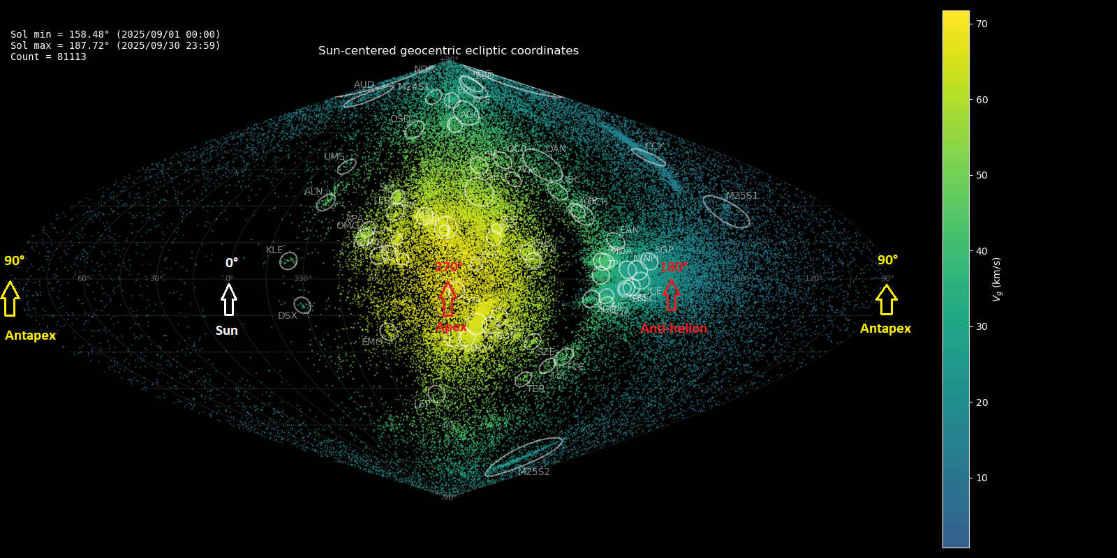
Figure 3 – GMN radiants for September 2025 plotted in Sun-centered Ecliptic Geocentric coordinates (SCE).
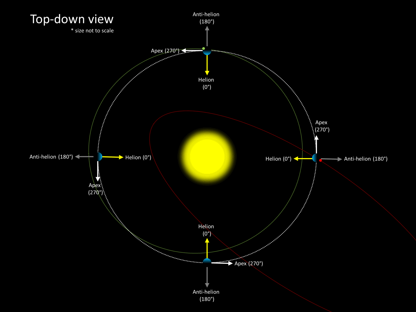
Figure 4 – Illustration of the Sun-centered ecliptic coordinate system with the Earth moving on its orbit in the direction of the Apex. (Credit GMN).
In meteor astronomy we use Sun-centered Ecliptic Geocentric coordinates (SCE), from the perspective of the Earth (geocentric), as opposed to the Sun (heliocentric). The Sun-centered part means that the coordinates are adjusted so that the Sun is always in the same place, at 0° in SCE longitude (Figure 4). The Sun-centered Geocentric Ecliptic Longitude is obtained by subtracting the Solar Longitude from the Geocentric Ecliptic Longitude and noted as λg – λʘ.
The best way to describe these coordinates is that they show the Earth’s “windshield”, knowing that the average orbital speed of the Earth around the Sun is approximately 29.78 km/s. Figure 3 shows the radiant distribution in Sun-centered Ecliptic Geocentric coordinates. The middle of the plot is the Earth’s apex – it’s direction of motion around the Sun. The reason why meteor speeds here are the highest is because we hit them head-on. 90° to the left is the Sun, and 90° to the right is the anti-helion direction. At 180° is our “back” and we see fewer meteors there because they have to catch up with the Earth so their apparent speeds are very slow.
This coordinate system is helpful because there is less radiant drift since the rotation of the Earth around the Sun is compensated. Most meteor shower radiants appear as fixed activity sources in Figure 3. Only a few radiants appear as elongated activity sources like the chi-Cygnids (CCY) where the radiant drift in Sun-centered Ecliptic Geocentric coordinates is caused by gradual changes in the meteoroid stream orbit orientation during Earth’s transit.
Most meteors are sporadics because they cannot be associated with any known meteoroid stream. GMN data has about 28% of meteors identified as belonging to meteor showers. These activities appear at the sky as a cluster of radiant points when the Earth crosses a trail of meteoroids moving around the Sun along a cometary or asteroidal orbit. Depending on the density of the dust concentration the number of shower meteors and related radiant points may be very distinct. Earth also intersects meteoroid streams at their outer edges where particles are irregularly and thinly distributed. Perceiving the presence of such activity embedded in the rich sporadic background is a matter of distinguishing between statistically relevant and spurious radiant concentrations.
5 Orbit data selection
Working with large datasets of millions of meteoroid orbits is rather slow and therefore we select only the orbits recorded during the activity period of a meteor shower.
As a first step all orbit data is selected during the expected activity period of the shower using the Solar Longitude. The limits of meteor shower activity are uncertain and can change with time. Therefore, adding one or two degrees in Solar Longitude to detect possible earlier or later activity than previously known can be useful. Solar Longitude makes it easy to combine data from different years. In some cases, the shower activity is studied for a specific year.
All available orbits are selected within the chosen range of time including both sporadic and shower meteoroid orbits. This is necessary to compare the shower activity to the sporadic background activity and to make specific distributions of orbital elements versus each other to evaluate the occurrence of orbit concentrations.
During the transit of the Earth through a meteoroid stream, the orientation of the Earth orbit relative to the direction of the meteoroid stream changes, resulting in a drift per day of the shower radiant at the sky. This motion of the Earth on its orbit can be compensated by using the Sun-centered ecliptic coordinates. All these coordinates are geocentric, relative to the Earth, including the Sun-centered coordinates and should not be confused with heliocentric coordinates, which are relative to the Sun.
To search for a possible concentration of orbits we need a reference orbit as a starting point for an iterative procedure to locate the best fitting mean orbit. To find such a start reference, we use the radiant position of the shower in Sun-centered geocentric ecliptic coordinates to select only those meteors that have their radiant within an estimated range in radiant position and velocity interval. The radiant position and size can be estimated from the radiant density maps. The velocity can be approached as the median velocity of this sample. This selection of meteors and their orbits consists mainly of shower meteors including a limited number of sporadics. The mean orbit for this selection is then computed using the method of Jopet et al. (2006). The resulting mean orbit serves as a first approach to find the best fitting mean orbit for all orbits that fit within a well-defined range of similarity.
6 Orbit discrimination criteria
We use the so-called similarity or discrimination or D-criteria to accept or to reject the identification of a shower meteoroid orbit. D-criteria are trying to put a number on how different two orbits are. D = 0 means the orbits are the same. The problem here is that using Keplerian orbital elements is tricky. The similarity criteria consider the distance between some of the orbital elements combined with the angle between the orbital planes. They’re trying to find a physically meaningful way to weight the differences, so that’s why we have different versions. The first numeric discrimination criterion was proposed by Southworth and Hawkins (1963), referred to as DSH. Later Drummond (1981) introduced a slightly different criterion, referred as DD. Jopek (1993) proposed another version DJ, based on the former criteria. We can apply all three criteria combined. Index p represents the reference orbit, index m the tested meteor orbit:
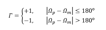
First, we determine the sign Γ, –1 or +1, as:
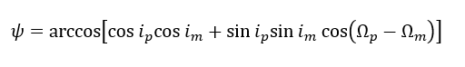
Then we calculate ψ, the angle between the two orbital planes from:
Next, we calculate Π, the angle between the perihelion points:
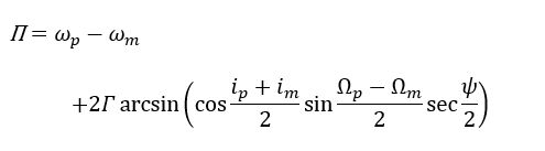
λ is the ecliptic longitude of the perihelion, with 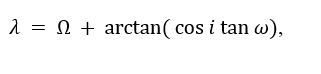
where λ has 180° added if cos ω < 0.
β is the ecliptic latitude of the perihelion, with
![]()
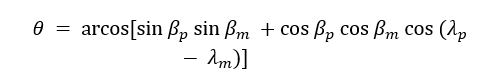
The angle θ between the two perihelion points on each orbit is given by the equation:
The three different discriminant criteria can now be calculated from the following equations, with DSH for the Southworth Hawkins criterion (1963), DD for the Drummond criterion (1981) and DJ for the Jopek criterion (1993):
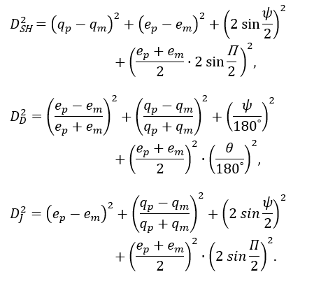
The larger the values of ψ, Π or θ, the bigger the ‘distances’ between the orbits and the less the probability becomes for an association. Related orbits have values in the order of a few degrees or less. The final values for these similarity criteria are dimensionless numeric values, where 0 represents identical orbits. The smaller the D-values the higher the degree of similarity and the better the probability becomes for an association. The D-criteria should be applied with caution. The result is a discriminant, without providing any proof for some physical relationship between the orbits. It is an approach in the sense of best effort and requires careful evaluation as the result highly depends upon the type of orbit.
Most meteor shower analyzers use arbitrary determined upper limits as a ‘safe’ threshold for the similarity criteria, typically DSH < 0.25 for Southworth and Hawkins and DD < 0.105 for Drummond. However, these thresholds are far too optimistic in most cases. Applying these values blindly leads to erroneous and confusing results. The most appropriate thresholds have to be considered on a case-by-case evaluation. A Rayleigh distribution fit on a sample of orbits under investigation helps to estimate the upper limit threshold in most cases. There are other methods to determine the optimal threshold for D-criteria some of which were published by Neslušan et al. (1995) and Rudawska et al. (2015).
Moreover, the D-criteria have specific shortcomings. The Southworth and Hawkins criterion has been criticized for being too dependent on the perihelion distance q. The Drummond criterion is too sensitive for the eccentricity e. The criterion defined by Jopek reduces the above-mentioned dependencies.
The purpose of identifying the best fitting orbit for a meteoroid stream is to eliminate sporadic look-alikes. Inappropriate use of D-criteria thresholds risks to result in a larger number of shower meteors but strongly affected by sporadic contamination. Therefore, we use the D-criteria of Southworth and Hawkins (1963), Drummond (1981) and Jopek (1993) combined. The results are considered in different classes of D-criteria thresholds with different degrees of similarity:
- Minimal: DSH < 0.25 & DD < 0.105 & DJ < 0.25.
- Poor: DSH < 0.2 & DD < 0.08 & DJ < 0.2.
- Medium poor: DSH < 0.15 & DD < 0.06 & DJ < 0.15.
- Medium: DSH < 0.125 & DD < 0.05 & DJ < 0.125.
- Medium high: DSH < 0.1 & DD < 0.04 & DJ < 0.1.
- Strong: DSH < 0.075 & DD < 0.03 & DJ < 0.075.
- Very strong: DSH < 0.05 & DD < 0.02 & DJ < 0.05.
- Best fit: DSH < 0.025 & DD < 0.01 & DJ < 0.025.
These classes should allow to compare shower characteristics in function of the reliability of the shower identification. While the poor threshold similarity classes may include sporadic orbits that fit the criteria by pure chance, the stronger the threshold the less the risk for contamination with sporadic orbits.
The reference orbit obtained as described in Section 4 is used to test against all orbits, regardless of their radiant position, by computing the three D-criteria thresholds for each orbit. Depending upon the type of orbit, the most appropriate D-criteria threshold class is used to select all orbits that fit within these threshold limits. A new mean orbit (Jopek et al., 2006) is computed for this selection which is used to repeat the procedure on a new selection of orbits where possibly sporadic orbits were removed. This iterative procedure stops when the set of selected orbits that fit the mean orbit doesn’t change anymore. Depending on the type of orbit the iteration procedure can be repeated for a more restricted class of D-criteria thresholds until it converges on a mean orbit as the best fit. All related meteor shower properties are derived from the mean orbit based on the final selection of shower meteor orbits.
If the initial reference orbit has been poorly determined the iteration can require many steps and skip away from the initial starting reference before the solution converges. In case a spurious activity source with unrelated orbits is investigated, the procedure runs idle unless it encounters another real activity source, if not, the iterations run into an endless loop.
6 Further analyses
The orbital parameters of all the meteors that fit a D-criteria threshold class can be used to make line graphs and diagrams for the entire time interval of activity. Orbital elements and velocity may display changes in function of time, expressed in Solar Longitude λʘ. These changes in orbit orientation during Earth’s transit results in a radiant drift in Sun-centered geocentric ecliptic coordinates.
The number of shower meteors relative to the number of non-shower meteors per unit of time can be used as an approximate activity profile for the shower. Different classes of D-criteria thresholds can be combined in such activity plot to compare the selection effect.
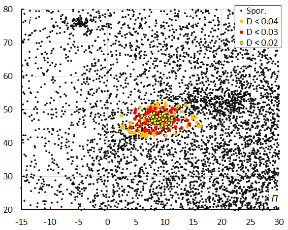
Figure 5 – The diagram of the inclination i against the longitude of perihelion Π color-coded for different classes of D criterion thresholds, for the October epsilon-Carinids in 2023–2025.
Frequently used plots are those of one orbital element versus another orbital element, such as inclination i versus longitude of perihelion Π. An example of the October epsilon-Carinids is given in Figure 5. These diagrams visualize the concentration in orbital elements with the non-shower meteors in the background and the investigated shower meteors color-code for different D-criteria threshold classes.
The type of the meteoroid orbit can be determined by the Tisserand parameter, TJ, with respect to Jupiter:
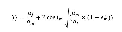
With aJ = 5.2044 A.U. In an ideal case, the following orbit types can be distinguished:
- TJ< 0.65 indicates a Long-period comet type orbit;
- 65 < TJ< 2.00 indicates a Mellish-type shower;
- 2.00 < TJ< 3.50 indicates a Jupiter family comet type orbit;
- TJ> 3.50 indicates an asteroid like type orbit.
In practice, there is a lot of intermixing. E.g. the biggest source of cometary dust in the Solar System is comet Encke, which is on a squarely asteroidal orbit. Further subdivision types have been defined within these classifications, but these main types of orbits are sufficient for the purpose of meteor shower analyses.
Table 1 – Main properties to define a meteor shower.
| λʘ (°) | Solar Longitude at maximum activity. |
| λʘb (°) | Solar Longitude at the start of the activity. |
| λʘe (°) | Solar Longitude at the end of the activity. |
| αg (°) | Geocentric right ascension in the J2000 epoch. |
| δg (°) | Geocentric declination in the J2000 epoch. |
| Δαg (°) | Radiant drift in Right Ascension. |
| Δδg (°) | Radiant drift in Declination. |
| vg (km/s) | Geocentric velocity. |
| Hb (km) | Begin height of the meteor. |
| He (km) | End height of the meteor. |
| Hp (km) | Height at which with peak magnitude occurred. |
| MagAp | Average peak mag. normalized at 100 km. |
| λg (°) | Geocentric ecliptic longitude in the J2000 epoch. |
| λg–λʘ(°) | Sun-centered geocentric ecliptic longitude. |
| βg (°) | Geocentric ecliptic latitude in the J2000 epoch. |
| a (A.U.) | Semi-major axis. |
| q (A.U.) | Perihelion distance. |
| e | Eccentricity. |
| i (°) | Inclination. |
| ω (°) | Argument of perihelion. |
| Ω (°) | Ascending node. |
| Π (°) | Longitude of perihelion. |
| Tj | Tisserand’s parameter with respect to Jupiter. |
| N | Number of meteors used for the mean orbit. |
The GMN procedure to identify meteor showers checks if a meteor is within the activity period, with a radiant within a changing radius of association from given coordinates (dispersion changes over time), and has speeds within a given range. The final result identifies a meteor shower with a list of physical parameters that distinguish the activity from other sources (Table 1). The meteoroid stream orbit is matched with all known minor bodies in our Solar System to locate any possible parent body.
7 Case study
As an example, we apply the method on a recently discovered meteor shower in Draco (M2025-Y1). This activity was first discovered during the night of December 12–13, 2025, by Belarusian and Ukrainian video camera networks (Harachka, 2026).
However, the likely radiant density maps of the GMN indicates that this activity started earlier and lasted longer than December 12–13, 2025. These maps serve as a first visual verification to estimate the activity duration and radiant location. The maps show a distinct activity from 8 until 15 December 2025, or 256° to 263° in Solar Longitude (Figures 7 and 8). Before applying the method for shower identification based on orbits we look at the results obtained by the method based on radiant identification.
7.1 Shower classification based on radiants
The GMN shower association criteria assume that meteors within 1° in Solar Longitude, within 4.9° in radiant in this case, and within 10% in geocentric velocity of a shower reference location are members of that shower. Further details about the shower association are explained in Moorhead et al. (2020). Using these meteor shower selection criteria, 263 meteors have been associated with the M2025-Y1 radiant in 2025, recorded by 414 cameras in Austria, Bosnia-Herzegovina, Belgium, Bulgaria, Canada, Croatia, Czech Republic, Denmark, Germany, Greece, France, Ireland, Italy, Netherlands, Portugal, Russia, Slovenia, South Korea, Spain, Switzerland, Ukraine, United Kingdom and the United States of America.
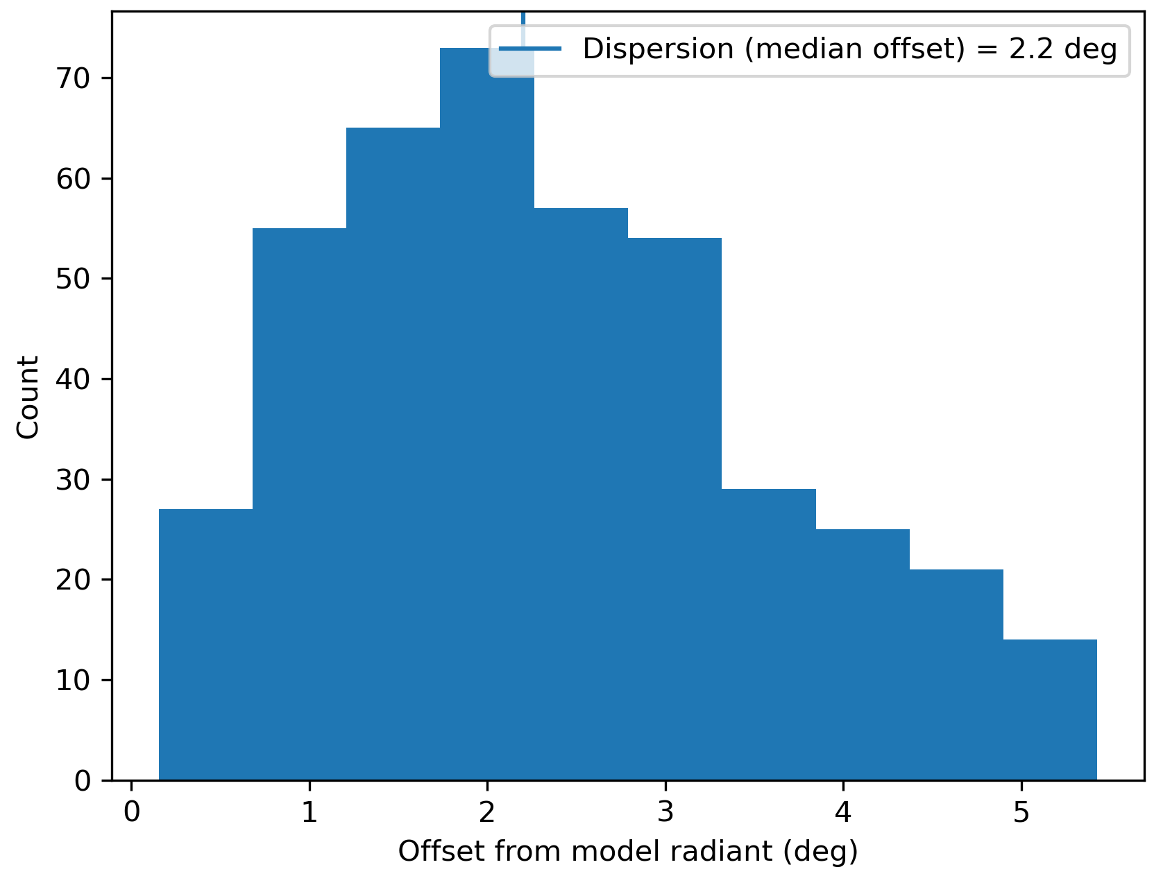
Figure 6 – Dispersion median offset on the radiant position.

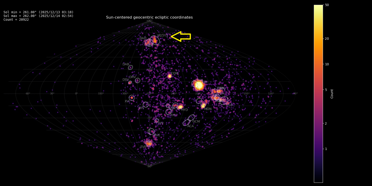
Figure 7 – Radiant density map with 20922 radiants obtained by the Global Meteor Network on 13–14 December, 2025. The position of the M2025-Y1 radiants in Sun-centered geocentric ecliptic coordinates is marked with a yellow arrow.
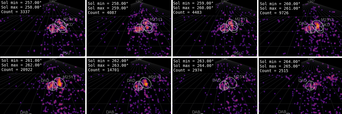
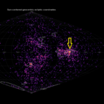
Figure 8 – Radiant density maps for 8–16 December 2025. The shower is labeled M25Y1.
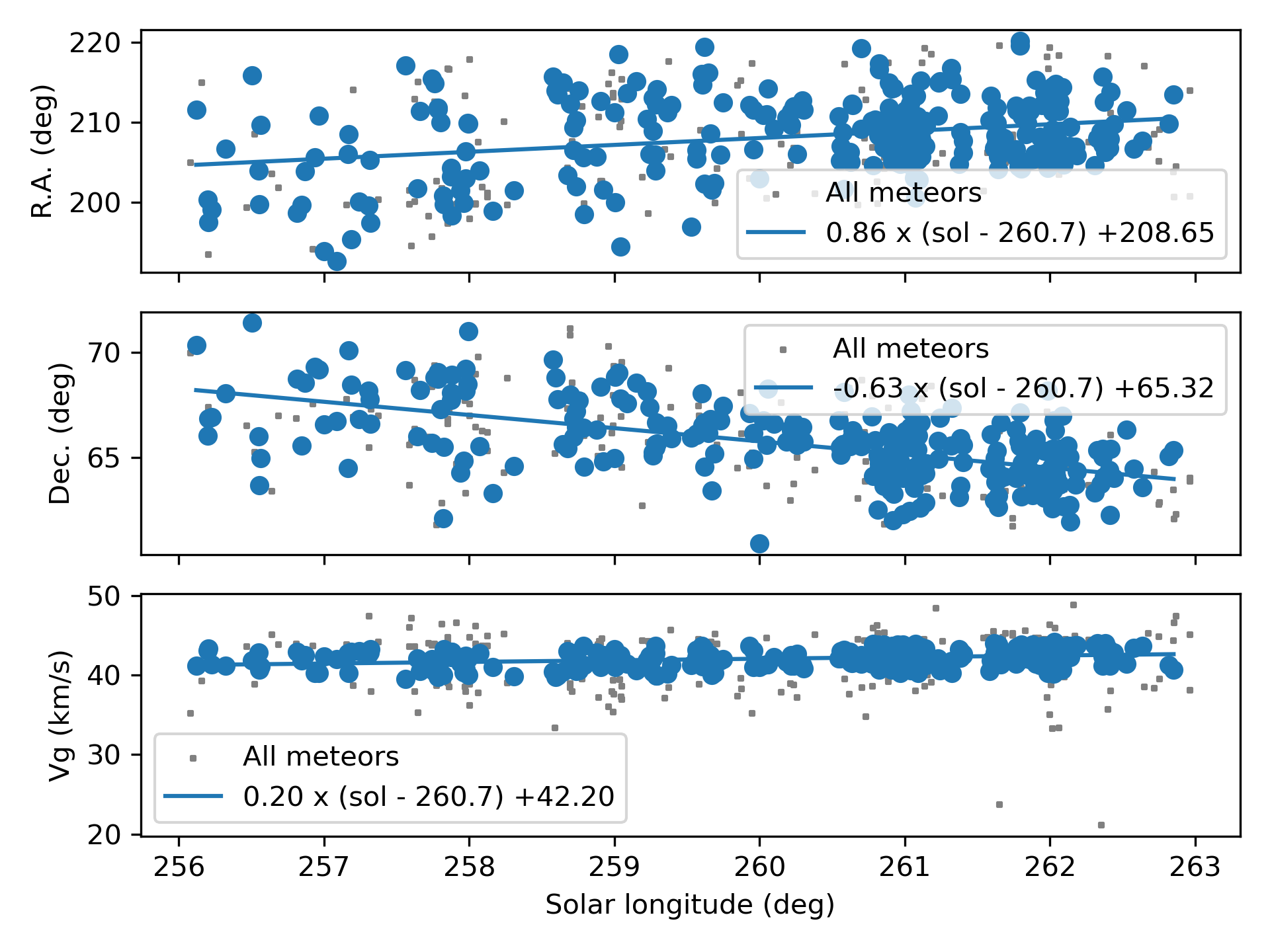
Figure 9 – The radiant drift.
This first shower identification method allows us to measure the radiant size (Figure 6), the radiant drift (Figure 9) and the number of M2025-Y1 meteors per degree in Solar Longitude (Figure 10).
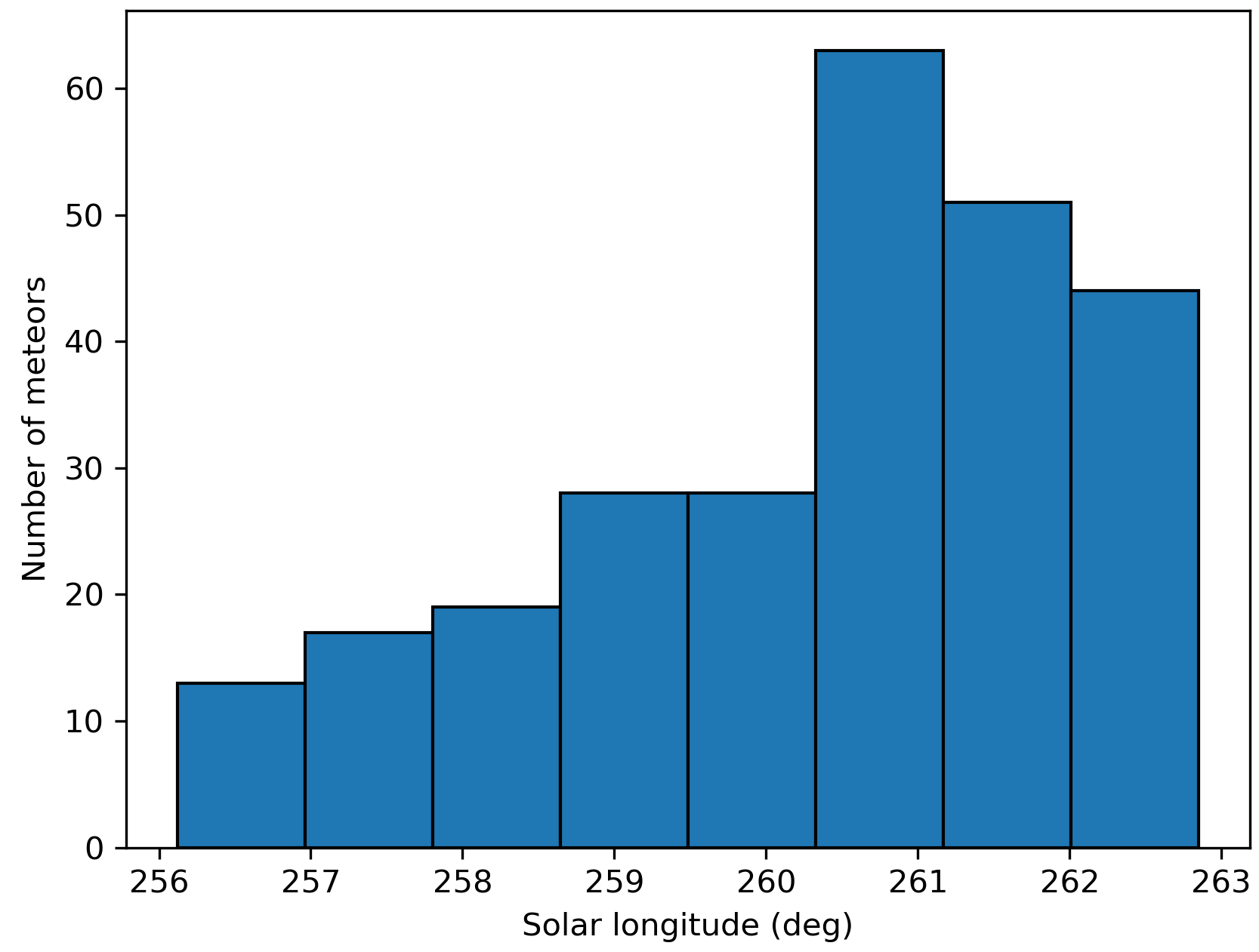
Figure 10 – The uncorrected number of shower meteors recorded per degree in solar longitude.
7.2 Shower classification based on orbits
The first step is to extract all orbit data from the GMN dataset available for the duration of the shower activity in Solar Longitude, 256° to 263°. For the years 2018 to 2025 there are 174427 orbits available within this interval. This selection will serve as a basis for the analysis.
To apply the similarity criteria, we need a first reference orbit to approach the best fitting orbit for M2025-Y1. From the radiant density maps we know the radiant position and the size of the radiant in Sun-centered ecliptic coordinates. We select all meteors that have their radiant within a radiant position roughly estimated from the maps at λ–λʘ ~ 252°±14° and β ~ +66°±6. This sample should include most of the M2025-Y1 meteors. Of the 174427 meteors selected between Solar Longitude 256° and 263°, 1279 have a radiant within these limits. We will use this sample to compute a first mean orbit for M2025-Y1 which will serve as a feed in the iterative procedure to locate orbits that fit within the thresholds of the discrimination criteria. The mean orbit is computed with the method described by Jopek et al (2006) using the Kepler elements q, e, i, Ω and ω. The 1279 selected orbits yield the following mean orbit:
- q = 0.958261 AU
- e = 0.804834
- i = 69.93924°
- Ω = 259.4143°
- ω = 196.1131°
This orbit is used as starting orbit and matched to all 174427 orbits selected between Solar Longitude 256° and 263°. This results in the following numbers of orbits fitting different D-criteria thresholds classes:
- DSH < 0.250 & DD < 0.105 & DJ < 0.250: 987 (G)
- DSH < 0.200 & DD < 0.080 & DJ < 0.200: 588 (F)
- DSH < 0.150 & DD < 0.060 & DJ < 0.150: 266 (E)
- DSH < 0.125 & DD < 0.050 & DJ < 0.125: 161 (D)
- DSH < 0.100 & DD < 0.040 & DJ < 0.100: 81 (C)
- DSH < 0.075 & DD < 0.030 & DJ < 0.075: 33 (B)
- DSH < 0.050 & DD < 0.020 & DJ < 0.050: 6 (A)
- DSH < 0.025 & DD < 0.010 & DJ < 0.025: 0 (A+)
These D-criteria do not prove any physical relationship and provide only a parameter that indicates how much two orbits differ. The smaller the value of D, the more similar the orbits are, the larger the value of D, the more difference between the orbit, the less the probability that there is any connection.
Historically, there has been too much confidence in these discrimination criteria and DSH < 0.250 was often considered as a safe cutoff to select orbits according to the Southworth and Hawkins D-criterion, or DD < 0.105 for the Drummond criterion. Caution is required as too optimistic cutoff values will include many sporadics that affect, or in some cases ruin, the final solution. The goal is to obtain reliable parameters that are representative for the meteoroid stream. In this perspective, it is better to have less outliers among the meteoroid stream members than to have a result that is contaminated by sporadics. Therefore, we do not use one single criterion but three different combined in order to filter away as many sporadics as possible. The threshold values strongly depend upon the type of orbit. The more sporadic orbits present in the sample used to derive a solution for the investigated meteor shower, the more uncertain the result.
It is recommended not to use the most optimistic cutoff values. The most suitable cutoff values can be derived by try-and-error. If the scatter on the resulting shower orbits is too large, the procedure should be repeated with lower threshold values. In practice it is a matter of experience based upon the type of orbit to pick the right threshold cutoff values. There are different methods to estimate the most relevant cutoff values, such as the Rayleigh fit applied on a set of Discrimination values for a specific criterion like the Drummond criterion for instance (Figure 11). In this particular case, the threshold class DSH < 0.125 & DD < 0.050 & DJ < 0.125 seems most suitable. We use these thresholds to select orbits.
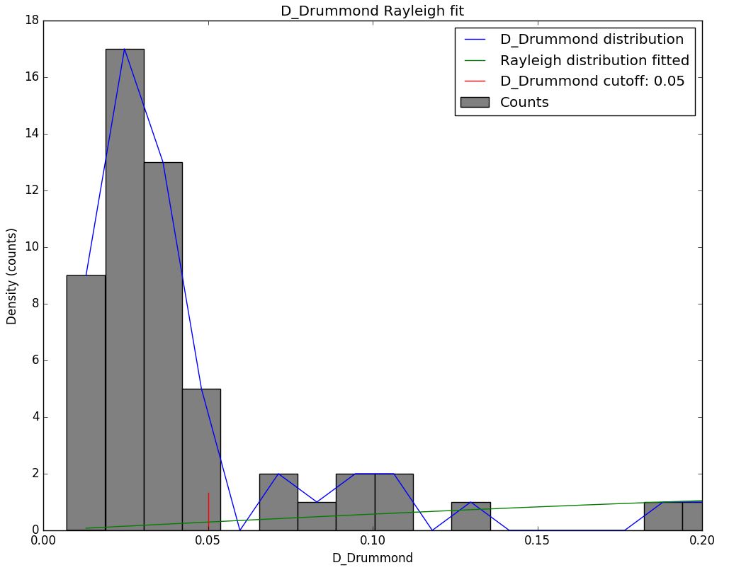
Figure 11 – Rayleigh fit on the Drummond criterion for M2025-Y1, 2025 data.
Table 2 – The Kepler elements for the mean orbit computed at each step in the iteration. The corresponding numbers of orbits that fit the criteria thresholds at each step is listed in Table 3.
| q | e | i | Ω | ω |
| 0.958261 | 0.804834 | 69.93924 | 259.4143 | 196.1131 |
| 0.963961 | 0.829654 | 70.19466 | 259.7787 | 196.0776 |
| 0.96386 | 0.856522 | 70.29293 | 259.9014 | 196.0051 |
| 0.96374 | 0.883708 | 70.50851 | 260.1155 | 195.9197 |
| 0.963282 | 0.899591 | 70.84129 | 260.0735 | 196.0455 |
| 0.963363 | 0.907387 | 71.08345 | 260.0901 | 196.0348 |
| 0.963446 | 0.911285 | 71.19059 | 260.0956 | 196.0331 |
| 0.963467 | 0.913492 | 71.22304 | 260.0843 | 196.0079 |
| 0.963445 | 0.914387 | 71.21668 | 260.07 | 196.0104 |
| 0.963529 | 0.91496 | 71.23434 | 260.0646 | 195.986 |
| 0.963488 | 0.91529 | 71.24994 | 260.0621 | 195.9995 |
| 0.963484 | 0.915391 | 71.26295 | 260.064 | 196.0078 |
| 0.963484 | 0.915391 | 71.26295 | 260.064 | 196.0078 |
The 161 orbits that fit this threshold class are selected and a new mean orbit is computed for this selection. This new mean orbit is matched again to the 174427 orbits resulting in 232 orbits that fit within the selected threshold class (D) (see Table 3). A new mean orbit is computed for these 232 orbits, and will be matched with all 174427 orbits. This way an iterative procedure is repeated until the Kepler elements of the obtained mean orbit (Table 2) and the number of orbits that fit the threshold class (Table 3) and do not change anymore. Then we assume we approached the best representative orbit for the cluster of orbits in our selection.
Table 3 – Evolution of the number of orbits among the sample of 174427 orbits that fit within the different threshold classes for the mean orbit computed at each step in the iteration.
| G | F | E | D | C | B | A | A+ |
| 987 | 588 | 266 | 161 | 81 | 33 | 6 | 0 |
| 988 | 674 | 376 | 232 | 140 | 55 | 12 | 0 |
| 963 | 715 | 481 | 357 | 208 | 101 | 27 | 0 |
| 932 | 716 | 521 | 416 | 296 | 167 | 46 | 4 |
| 922 | 709 | 529 | 423 | 319 | 189 | 58 | 6 |
| 916 | 707 | 526 | 424 | 318 | 203 | 75 | 9 |
| 909 | 706 | 521 | 425 | 320 | 201 | 77 | 6 |
| 909 | 704 | 519 | 428 | 324 | 200 | 77 | 6 |
| 903 | 703 | 517 | 428 | 327 | 197 | 77 | 8 |
| 903 | 702 | 517 | 430 | 326 | 197 | 76 | 8 |
| 903 | 701 | 514 | 429 | 327 | 197 | 76 | 8 |
| 903 | 702 | 513 | 429 | 328 | 198 | 77 | 8 |
| 903 | 702 | 513 | 429 | 328 | 198 | 77 | 8 |
Table 2 lists the Kepler elements of each mean orbit at each step of the iteration and Table 3 the corresponding number of orbits that fit within the different threshold classes for these mean orbits for the entire loop of iterations. It is obvious that the starting mean orbit based upon the 1279 meteors that have their radiant within the selected zone included many sporadics and other shower meteors since most of these 1279 meteors don’t fit within the threshold values. The number of fitting orbits increases rapidly with each step in the iteration while the cluster of M2025-Y1 orbits is being approached and sporadic orbits being rejected. After twelve steps, 429 orbits fit the threshold class DSH < 0.125 & DD < 0.050 & DJ < 0.125 and this number (Table 3) nor the Kepler elements (Table 2) change any further. At this step we conclude that the last mean orbit represents the best fitting solution for the cluster of M2025-Y1 orbits.
The choice of the start orbit for the iteration determines how many steps are needed to approach the best fitting mean orbit. In some cases, it may take only a few steps. If a spurious concentration is searched, the process keeps skipping around. For new activity sources, an estimated radiant area can be used like in the example above. In most cases the GMN orbit data includes a shower association based on known radiant positions. It is possible to derive a mean orbit based upon the GMN shower identification. The GMN orbit dataset has such identification for M2025-Y1 with 370 meteors identified with this new shower in 2025. Table 4 lists the Kepler elements at each iteration step using the mean orbit for these 370 M2025-Y1 meteors in the dataset in order to find a solution for 2025 data only.
Table 4 – The Kepler elements for the mean orbit computed at each step in the iteration for 2025 data.
| q | e | i | Ω | ω |
| 0.963691 | 0.883078 | 69.97857 | 260.3954 | 195.4147 |
| 0.964512 | 0.896789 | 70.47772 | 260.4274 | 195.5483 |
| 0.964491 | 0.901948 | 70.74938 | 260.4275 | 195.5974 |
| 0.964493 | 0.905516 | 70.89979 | 260.4216 | 195.6042 |
| 0.964508 | 0.907729 | 70.97995 | 260.4322 | 195.6119 |
| 0.964606 | 0.908574 | 70.97657 | 260.441 | 195.5711 |
| 0.964682 | 0.909495 | 70.99641 | 260.4612 | 195.5405 |
| 0.964698 | 0.910116 | 71.01583 | 260.4589 | 195.5319 |
| 0.9647 | 0.910762 | 71.00023 | 260.4503 | 195.5205 |
| 0.964657 | 0.911412 | 70.99261 | 260.4419 | 195.5318 |
| 0.964657 | 0.911412 | 70.99261 | 260.4419 | 195.5318 |
Table 5 – Evolution of the number of orbits among the sample of 174427 orbits that fit within the different threshold classes for the mean orbit computed at each step in the iteration for 2025 data.
| G | F | E | D | C | B | A | A+ |
| 434 | 354 | 292 | 249 | 187 | 101 | 32 | 2 |
| 425 | 361 | 299 | 258 | 193 | 118 | 42 | 3 |
| 425 | 360 | 299 | 258 | 194 | 124 | 45 | 6 |
| 421 | 359 | 298 | 258 | 190 | 123 | 50 | 7 |
| 423 | 359 | 299 | 257 | 190 | 122 | 53 | 6 |
| 422 | 358 | 299 | 258 | 190 | 120 | 52 | 7 |
| 424 | 359 | 299 | 256 | 190 | 119 | 51 | 6 |
| 424 | 359 | 299 | 256 | 192 | 119 | 51 | 6 |
| 424 | 359 | 299 | 254 | 191 | 118 | 51 | 6 |
| 424 | 359 | 298 | 254 | 192 | 117 | 51 | 7 |
| 424 | 359 | 298 | 254 | 192 | 117 | 51 | 7 |
For 2025 data, 254 orbits fit the DSH < 0.125 & DD < 0.050 & DJ < 0.125 threshold values. It is obvious that an outburst occurred in 2025 as previous years had far less M2025-Y1 candidates although that this part of the sky was well covered by GMN in previous years. The number of shower meteors identified using the orbit classification method is much smaller than the 370 M2025-Y1 meteors identified by the radiant classification method.
7.3 Complete example of an in-depth analysis
The two solutions, one for 2025 and one for 2018–2025, make it possible to extract records from the GMN dataset for different threshold classes to make graphics and to compare all meteor shower parameters. In Table 6, the results obtained by the orbit identification method, described above, are compared to the result of the radiant based identification method. The plot of the radiant positions in Figure 12 clearly shows the cluster of M2025-Y1 radiants. Another concentration is visible just south of the M2025-Y1 radiant, the December alpha-Draconids (DAD#334). Right of the M2025-Y1 radiant and partly mixed with it are the December kappa-Draconids, DKD#336.
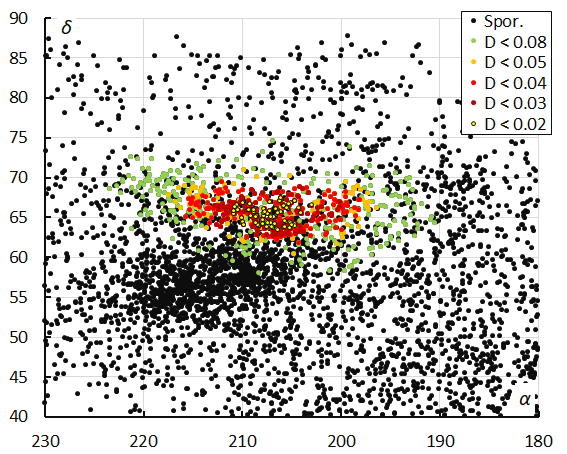
Figure 12 – The radiant distribution during the solar-longitude interval 256° – 263° in equatorial coordinates, color-coded for different threshold values of the combined similarity criteria.
Table 6 – Comparing solutions for M2025-Y1 derived by the radiant based method and the orbit based method for
DSH < 0.125 & DD < 0.050 & DJ < 0.125 for 2025 data, both compared to 2019–2025 data and the December kappa-Draconids, DKD#336 (Jenniskens, 2023).
| Radiant method
2025 |
Orbit method 2025 | Orbit method 2019-25 | DKD #336 | |
| λʘ (°) | 260.7 | 260.9 | 260.6 | 251.2 |
| λʘb (°) | 256.0 | 256.2 | 256.1 | 244 |
| λʘe (°) | 263.0 | 262.9 | 263.0 | 261 |
| αg (°) | 208.6 | 207.5 | 206.7 | 187.1 |
| δg (°) | +65.3 | +65.4 | +65.5 | +69.9 |
| Δαg (°) | +0.86 | +0.97 | +1.03 | +1.05 |
| Δδg (°) | –0.63 | –0.64 | –0.65 | –0.50 |
| vg (km/s) | 42.2 | 42.9 | 43.0 | 43.5 |
| Hb (km) | 105.0 | 105.4 | 105.6 | 107.7 |
| He (km) | 94.6 | 94.5 | 94.1 | 93.3 |
| Hp (km) | 99.4 | 99.2 | 99.2 | 98.5 |
| MagAp | –0.1 | –0.25 | –0.3 | 0.0 |
| λg (°) | 153.93 | 154.3 | 153.54 | 135.6 |
| λg – λʘ (°) | 253.23 | 253.2 | 252.9 | 244.4 |
| βg (°) | +65.93 | +65.3 | +65.1 | +61.7 |
| a (A.U.) | 8.577 | 10.9 | 11.4 | 9.01 |
| q (A.U.) | 0.965 | 0.965 | 0.964 | 0.930 |
| e | 0.887 | 0.911 | 0.915 | 0.897 |
| i (°) | 70.2 | 71.0 | 71.3 | 72.9 |
| ω (°) | 195.4 | 195.5 | 196.0 | 208.2 |
| Ω (°) | 260.3 | 260.4 | 260.1 | 251.2 |
| Π (°) | 95.8 | 96.0 | 96.1 | 99.7 |
| Tj | 1.01 | 0.87 | 0.84 | 0.89 |
| N | 263 | 254 | 429 | 1982 |
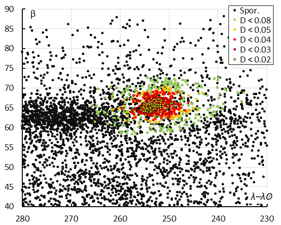
Figure 13 – The radiant distribution during the solar-longitude interval 256° – 263° in Sun-centered geocentric ecliptic coordinates, color-coded for different threshold values of the combined similarity criteria.
The radiant plot in Sun-centered geocentric ecliptic coordinates neutralizes the radiant drift caused by the movement of the Earth on its orbit around the Sun. The large scatter on radiants for DSH < 0.2 & DD < 0.08 & DJ < 0.2 indicates that these threshold values are too tolerant. Figure 13 shows a very dense cluster of M2025-Y1 radiants. At left is the concentration of the December alpha-Draconids and at right are December kappa-Draconids radiants. This shower had its maximum nine days before M2025-Y1, but the end of its activity period overlaps with the first days of the M2025-Y1 activity. Several M2025-Y1 orbits had been initially classified as December kappa-Draconids. The meteoroid stream parameters of this shower are added to Table 6 as these resemble a lot to those of M2025-Y1.
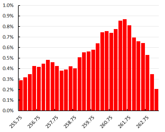
Figure 14 – The percentage of M2025-Y1-meteors relative to the total number of meteors without the Geminids.
The percentage of M2025-Y1 meteors relative to the total number of meteors provides a way to reconstruct an activity profile. As one of the richest meteor showers of the year – the Geminids – had their maximum during this time interval, the Geminids were disregarded. Although the median value for the Solar Longitude is 260.7°, there is no real peak activity but enhanced activity for about two days.
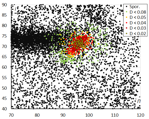
Figure 15 – The diagram of the inclination i versus the longitude of perihelion Π color-coded for different classes of D-criteria thresholds, for λʘ between 256° and 263°.
Apart from radiant plots, diagrams with Kepler elements plotted versus each other is a useful way to visualize clusters with similar orbital elements. One of the most suitable combinations is the inclination versus Longitude of Perihelion. In Figure 15 the M2025-Y1 concentration is very well visible. At the left of it, the December alpha-Draconids. Next to the M2025-Y1 cluster and partially intermixed are the December kappa-Draconids, suggesting that there is a likely relationship between M2025-Y1 and the December kappa-Draconids.
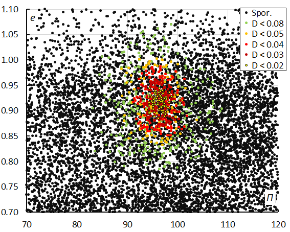
Figure 16 – The diagram of the eccentricity e versus the longitude of perihelion Π color-coded for different classes of D-criteria thresholds, for λʘ between 256° and 263°.
Depending on the type of orbits meteoroid streams appear as distinct clusters in these diagrams. Different clusters are visible in Figures 16 to 19, caused by different meteor showers such as e-Velids (EVE#746), alpha-Canis Majorids (ACA#394), gamma-Canis Majorids (GCM#395), etc. One particular activity source appears close to the M2025-Y1 or partly mixed in its cluster, the December kappa-Draconids (DKD#336). This suggests a physical connection between M2025-Y1 and the December kappa-Draconids. A sample of December kappa-Draconids has been taken from the 2024 GMN data for comparison.
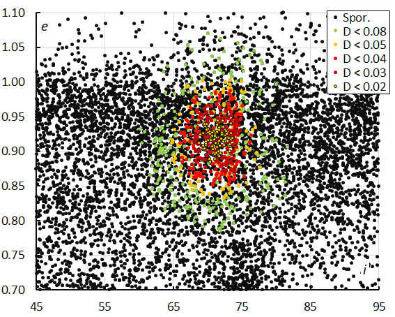
Figure 17 – The diagram of the eccentricity e versus the inclination i color-coded for different classes of D-criteria thresholds, for λʘ between 256° and 263°.
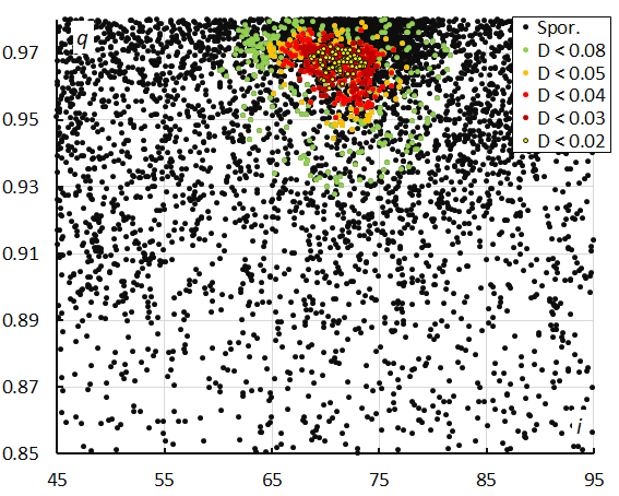
Figure 18 – The diagram of the perihelion distance q versus the inclination i color-coded for different classes of D-criteria thresholds, for λʘ between 256° and 263°.
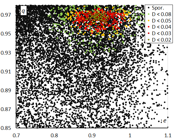
Figure 19 – The diagram of the perihelion distance q versus the eccentricity e color-coded for different classes of D-criteria thresholds, for λʘ between 256° and 263°.
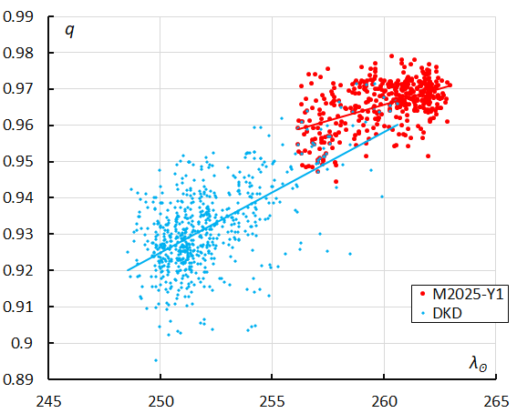
Figure 20 – The evolution of the perihelion distance q in function of the Solar Longitude λʘ for the M2025-Y1 orbits (2019–2025) and December kappa-Draconids (2024).
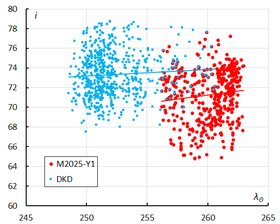
Figure 21 – The evolution of the inclination i in function of the Solar Longitude λʘ for the M2025-Y1 orbits (2019–2025) and December kappa-Draconids (2024).
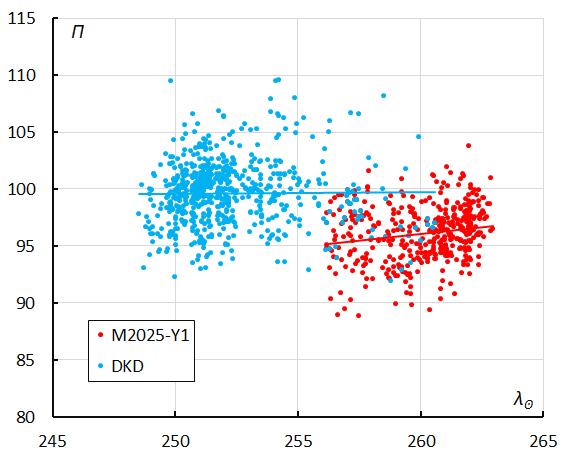
Figure 22 – The evolution of the Longitude of Perihelion Π in function of the Solar Longitude λʘ for the M2025-Y1 orbits (2019–2025) and December kappa-Draconids (2024).
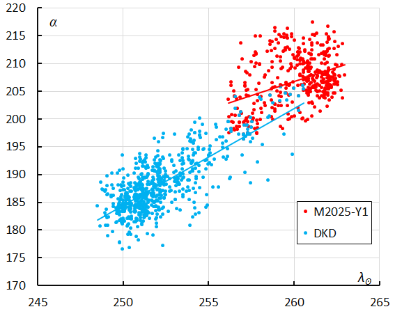
Figure 23 – The radiant drift in Right Ascension α in function of the Solar Longitude λʘ for the M2025-Y1 orbits (2019–2025) and December kappa-Draconids (2024).
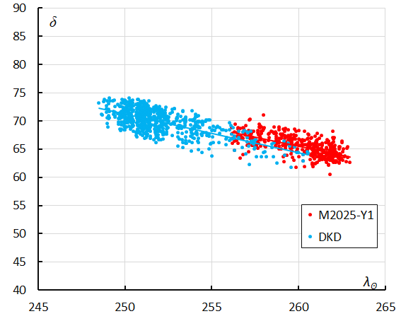
Figure 24 – The radiant drift in Declination δ in function of the Solar Longitude λʘ for the M2025-Y1 orbits (2019–2025) and December kappa-Draconids (2024).
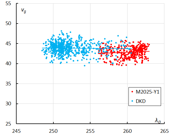
Figure 25 – The geocentric velocity vg in function of the Solar Longitude λʘ for the M2025-Y1 orbits (2019–2025) and December kappa-Draconids (2024).
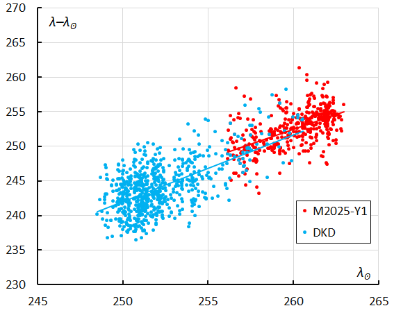
Figure 26 – The Sun-centered geocentric longitude λ–λʘ in function of the Solar Longitude λʘ for the M2025-Y1 orbits (2019–2025) and December kappa-Draconids (2024).
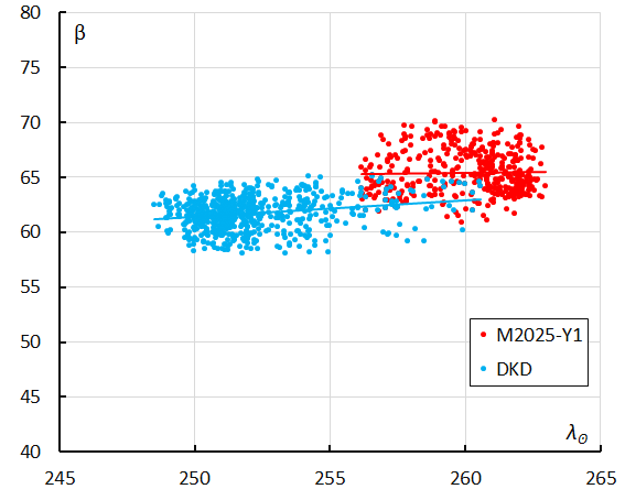
Figure 27 – The geocentric latitude β in function of the Solar Longitude λʘ for the M2025-Y1 orbits (2019–2025) and December kappa-Draconids (2024).
The distributions for different parameters in function of time (λʘ) show a likely link between M2025-Y1 and the December kappa-Draconids. The perihelion distance q increases during the activity period and where the final days of activity for the DKD ends, M2025-Y1 starts (Figure 20). The same for inclination i (Figure 21) and Longitude of Perihelion Π (Figure 22) with a small offset in position.
The radiant positions in Right Ascension (Figure 23) and Declination (Figure 24) visualize the radiant drift caused by the movement of the Earth. The radiant drift at the end of the activity of the December kappa-Draconids overlaps with the start of the M2025-Y1 activity and displays a similar trend. The geocentric velocity is comparable (Figure 25). The radiant drift in Sun-centered geocentric coordinates is caused by changes in the orientation of the orbital plane during Earth’s transit through the meteoroid stream. The December kappa-Draconids and M2025-Y1 align very well in Figures 26 and 27.
The Tisserand value relative to Jupiter TJ = 0.84 is a Halley-type comet orbit with a subclassification as a Mellish-type shower. This is very close to the value for the December kappa-Draconids which have TJ = 0.89±0.52 (Jenniskens, 2023). Jenniskens associates the December kappa-Draconids with comet 12P/Pons-Brooks.
A search for possible parent bodies for the M2025-Y1 orbit resulted in the ten best matches listed in Table 7 with comet 12P/Pons-Brooks as most likely candidate, the same parent body of the December kappa-Draconids. The M2025-Y1 orbit fits with the 12P/Pons-Brooks orbit with DSH = 0.21 & DD = 0.11 & DJ = 0.14, the DKD#336 orbit fits with DSH = 0.21 & DD = 0.10 & DJ = 0.17. Figure 28 shows the three highly inclined orbits in space.
Table 7 – Top ten matches of a search for possible parent bodies with DD < 0.27, based upon the mean orbit derived from the radiant classification method.
| Name | DD |
| 12P/Pons-Brooks | 0.12 |
| C/1785 A1 (Messier-Mechain) | 0.132 |
| 8P/Tuttle | 0.15 |
| C/1898 L2 (Perrine) | 0.228 |
| C/1975 X1 (Sato) | 0.231 |
| C/1991 Y1 (Zanotta-Brewington) | 0.238 |
| C/2012 V2 (LINEAR) | 0.243 |
| C/2012 L2 (LINEAR) | 0.248 |
| C/2010 G1 (Boattini) | 0.259 |
| (369264) 2009 MS | 0.262 |
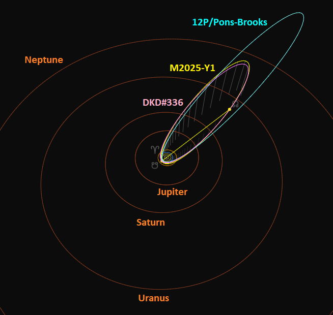
Figure 28 – Comparing the M2025-Y1 solution (yellow) and the December kappa-Draconids (DKD#336) (pink) with the orbit of the most likely parent body 12P/Pons-Brooks (blue). (Plotted with the Orbit visualization app provided by Pető Zsolt).
The DKD#336 orbit intersects the Earth orbit at its descending node shortly before the M2025-Y1 orbit intersects the Earth orbit. The descending node of comet 12P/Pons-Brooks crosses the ecliptic inside the Earth orbit (Figure 29). The object is classified as a Near Earth Asteroid (NEA). The comet was discovered in July 1812 at Marseilles Observatory by the French astronomer Jean-Louis Pons and was rediscovered by the British-American astronomer William Robert Brooks in 1883, it received the name Pons-Brooks. With its orbital period of 71.491 years, it reoccurred on 20 June 1953. The comet has a nucleus about 34 km in diameter. Older observations were related to this comet in 1385 and 1457. Its most recent perihelion passage took place on April 21, 2024.
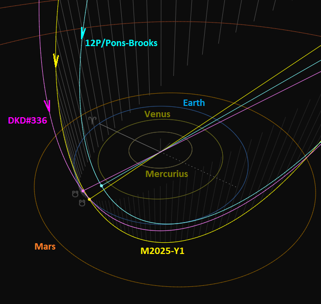
Figure 29 – Comparing the M2025-Y1 solution (yellow) and the December kappa-Draconids (DKD#336) (pink) with the orbit of the most likely parent body 12P/Pons-Brooks (blue), close-up at the inner Solar System. (Plotted with the Orbit visualization app provided by Pető Zsolt).
Belarusian and Ukrainian video meteor networks obtained a spectrum of a M2025-Y1 meteor which belongs to the Fe-poor type. Meteoroids of this type are rich in magnesium and have a normal sodium content, but poor iron content. This is typical for meteoroids with Halley-type orbits (Harachka, 2026). This is different from the spectral type cited by Jenniskens (2023) where December kappa-Draconids are listed as Na poor/free, based on research by Matlovič et al. (2019).
The appearance of a meteor activity outburst, initially considered as a possible new meteor shower, could be linked to the known December kappa-Draconids and the parent object 12P/Pons-Brooks. The outburst occurred after the known end of the activity period of this shower and must have been caused by an unknown dust trail related to the parent body which passed its perihelion in April 2024. In previous years far less possible M2025-Y1 meteors were counted: zero in 2018; two in 2019, three in 2020, nine in 2021, 28 in 2022, 64 in 2023, 71 in 2024 and 252 in 2025. The numbers partially represent the expansion of the GMN network but the outburst in 2025 is clearly the result of an encounter with a dust trail.
8 Conclusion
Meteoroid orbit data offer a completely different gamma of possibilities for meteor shower analyses than what was possible before statistical relevant datasets with meteoroid orbits became available. Amateurs focused their meteor shower analyses on visual observing data for major showers. Minor showers suffered from the uncertainty in radiant determination by single station visual observers and small number statistics. The large numbers of meteoroid orbits obtained by low-light camera networks make it possible to unravel weak activity sources. So far, very few amateurs gained expertise in this field where many discovered but unconfirmed activity sources wait for analyses that can help to document these meteor showers and get them confirmed as established shower in the IAU-MDC Working List of Meteor Showers.
This publication explains the method to identify shower meteors using D-criteria on meteoroid orbits. The method is demonstrated with an analysis of the possible new meteor shower M2025-Y1 that was discovered in December 2025. The ‘new’ meteor shower has the same characteristics as the minor annual shower December kappa-Draconids and appears to have been produced by an unknown dust trail beyond the known activity period of the December kappa-Draconids.
The authors recommend the IAU-MDC to move the entry for M2025-Y1 as a new solution for the December kappa-Draconids. Comet 12P/Pons-Brooks should be listed as parent body.
Acknowledgments
This report is based on the data of the Global Meteor Network (Vida et al., 2020a; 2020b; 2021) which is released under the CC BY 4.0 license. We thank all 927 participants in the Global Meteor Network project for their contribution and perseverance. A list with the names of the volunteers who contribute to GMN has been published in the 2025 annual report (Roggemans et al., 2026). The following 760 cameras contributed to paired meteors used in this study:
AT0004, BA0001, BA0002, BA0003, BA0004, BA0005, BE0001, BE0003, BE0004, BE0005, BE0006, BE0007, BE0008, BE0009, BE000B, BE000C, BE000E, BE000G, BE000H, BE000K, BE000L, BE000M, BE000Q, BE000S, BE000T, BE000U, BE000V, BE000W, BE000X, BE000Y, BE000Z, BE0010, BE0011, BE0013, BE0014, BE0017, BE0018, BE0019, BE001A, BG0001, BG0003, BG0009, BG000A, BG000B, BG000C, BG000F, BG000G, BG000H, BG000J, CA000F, CA000Q, CA000U, CA000V, CA001F, CA001R, CA001X, CA0023, CA002F, CA002K, CA002L, CA002N, CA0031, CA0037, CA003A, CA003B, CA003C, CA003D, CAWEC1, CH0003, CH0004, CH0005, CZ0003, CZ0004, CZ0006, CZ0007, CZ0008, CZ000A, CZ000F, CZ000H, CZ000J, CZ000L, CZ000M, CZ000P, CZ000R, CZ000W, CZ000X, DE0001, DE0002, DE0004, DE0005, DE0006, DE0007, DE0009, DE000B, DE000G, DE000J, DE000K, DE000M, DE000Q, DE000S, DE000W, DE000X, DE000Y, DE0011, DE0012, DE0013, DE0015, DE0016, DK0001, DK0003, DK0006, DK0009, DK000J, DK000L, DK000M, DK000Q, DK000R, DK000T, ES0001, ES0002, ES0003, ES0004, ES0005, ES0009, ES000D, ES000F, ES000H, ES000Q, ES000T, ES000U, ES000V, ES000X, ES0013, ES0016, ES0019, ES001A, ES001F, FR0003, FR0006, FR000A, FR000F, FR000R, FR000U, FR000X, FR000Y, FR000Z, FR0011, FR0013, FR0014, GR0002, GR0003, GR0004, GR0005, GR0006, GR0007, GR0008, GR0009, HR0001, HR0002, HR0006, HR0007, HR0008, HR000D, HR000J, HR000P, HR000Q, HR000S, HR000U, HR000V, HR000W, HR0010, HR0015, HR001D, HR001E, HR001J, HR001K, HR001M, HR001R, HR001V, HR001X, HR001Z, HR0025, HR0027, HR002D, HR002E, HR002F, HR002G, HR002H, HR002J, HR002K, HR002R, HR002T, HR002V, HR002W, HR002X, HR002Y, HU0002, HU0003, IE0004, IE000G, IE000H, IE000J, IE000M, IL0002, IL0008, IL0009, IL000A, IT0001, IT0004, IT0007, IT0008, IT000A, IT000B, KR0002, KR0004, KR0006, KR0007, KR0009, KR000A, KR000B, KR000C, KR000D, KR000E, KR000F, KR000G, KR000H, KR000J, KR000K, KR000L, KR000M, KR000N, KR000P, KR000Q, KR000R, KR000S, KR000V, KR000Y, KR0010, KR0011, KR0013, KR0014, KR0015, KR0016, KR0017, KR0018, KR0019, KR001A, KR001B, KR001C, KR001E, KR001H, KR001K, KR001L, KR001M, KR001X, KR001Y, KR001Z, KR0020, KR0021, KR0022, KR0023, KR0024, KR0025, KR0026, KR0027, KR0028, KR0029, KR002A, KR002B, KR002C, KR002D, KR002E, KR002F, KR002G, KR002L, KR002M, KR002P, KR002Q, KR002R, KR002S, KR0036, KR0037, KR003A, KR003J, KR003L, KR003M, KR003N, KR003P, KR003Q, KR003R, KR003S, KR003T, KR003U, KR003V, KR003W, KR003X, LU0001, MX000D, NL0001, NL0006, NL0009, NL000A, NL000B, NL000C, NL000D, NL000G, NL000K, NL000M, NL000N, NL000P, NL000Q, NL000R, NL000S, NL000T, NL000U, NL000Z, NL0011, NL0013, NL0014, NL0017, NL0019, NL001E, PT0002, PT0003, RU0001, RU0003, RU0004, RU0008, RU0009, RU000E, RU000F, RU000M, RU000N, RU000Q, RU000T, RU000Y, RU0016, RU0017, RU0018, RU0019, SI0001, SI0002, SI0003, SI0004, SI0005, SI0006, SK0002, SK0003, SK0004, SK0005, SK0006, UA0001, UA0002, UK0001, UK0004, UK0006, UK0008, UK0009, UK000B, UK000D, UK000F, UK000H, UK000J, UK000P, UK000S, UK000T, UK000U, UK000Y, UK000Z, UK001E, UK001H, UK001K, UK001L, UK001M, UK001N, UK001P, UK001Q, UK001R, UK001S, UK001T, UK001U, UK001V, UK001W, UK001Z, UK0021, UK0022, UK0024, UK0025, UK0026, UK0027, UK002F, UK002J, UK002K, UK002L, UK002Q, UK002S, UK002T, UK002W, UK002X, UK002Z, UK0030, UK0031, UK0032, UK0034, UK0035, UK0039, UK003A, UK003B, UK003C, UK003D, UK003E, UK003F, UK003L, UK003N, UK003T, UK003U, UK003V, UK003W, UK003X, UK003Y, UK003Z, UK0041, UK0042, UK0045, UK0049, UK004B, UK004C, UK004D, UK004E, UK004F, UK004G, UK004J, UK004M, UK004N, UK004P, UK004U, UK004V, UK0050, UK0051, UK0055, UK0057, UK005C, UK005E, UK005G, UK005H, UK005J, UK005L, UK005M, UK005N, UK005P, UK005R, UK005S, UK005U, UK005V, UK0061, UK0062, UK0063, UK0066, UK0067, UK006A, UK006B, UK006C, UK006D, UK006G, UK006J, UK006L, UK006P, UK006Q, UK006S, UK006T, UK006U, UK006V, UK006X, UK006Z, UK0070, UK0072, UK0073, UK0074, UK0077, UK0078, UK0079, UK007A, UK007B, UK007C, UK007E, UK007G, UK007H, UK007J, UK007L, UK007N, UK007P, UK007Q, UK007R, UK007U, UK007V, UK007Y, UK007Z, UK0080, UK0081, UK0082, UK0083, UK0084, UK0085, UK0086, UK0087, UK0088, UK0089, UK008A, UK008B, UK008C, UK008D, UK008E, UK008F, UK008G, UK008H, UK008J, UK008Q, UK008R, UK008S, UK008T, UK008U, UK008V, UK008X, UK008Z, UK0090, UK0092, UK0096, UK0098, UK0099, UK009A, UK009C, UK009D, UK009F, UK009G, UK009J, UK009K, UK009L, UK009M, UK009P, UK009Q, UK009R, UK009S, UK009T, UK009U, UK009V, UK009W, UK009X, UK00A0, UK00A1, UK00A2, UK00A3, UK00A4, UK00A5, UK00A6, UK00A7, UK00AA, UK00AB, UK00AD, UK00AE, UK00AF, UK00AG, UK00AJ, UK00AK, UK00AL, UK00AM, UK00AN, UK00AP, UK00AQ, UK00AS, UK00AT, UK00AU, UK00B0, UK00B1, UK00B2, UK00B5, UK00B6, UK00BA, UK00BB, UK00BC, UK00BH, UK00BJ, UK00BK, UK00BL, UK00BN, UK00BQ, UK00BW, UK00C0, UK00C1, UK00C2, UK00C3, UK00C4, UK00C6, UK00C7, UK00C9, UK00CA, UK00CC, UK00CD, UK00CE, UK00CH, UK00CJ, UK00CK, UK00CQ, UK00CS, UK00CT, UK00CU, UK00CV, UK00CZ, UK00D7, UK00D9, UK00DA, UK00DB, UK00DD, UK00DE, UK00DG, UK00DH, UK00DJ, US0001, US0002, US0003, US0004, US0005, US0006, US0007, US0008, US0009, US000A, US000C, US000D, US000E, US000G, US000H, US000J, US000K, US000L, US000M, US000N, US000P, US000R, US000S, US000U, US000V, US0019, US001E, US001G, US001L, US001N, US001P, US001Q, US001R, US001U, US001V, US0020, US0021, US0022, US0023, US0026, US0027, US002A, US002D, US002E, US002J, US002L, US002M, US002N, US002P, US002Q, US002R, US002W, US002X, US002Y, US0030, US0035, US0036, US0037, US0038, US0039, US003G, US003M, US003N, US003P, US003Q, US003R, US003S, US003T, US003Y, US0040, US0043, US0044, US0045, US004B, US004C, US004D, US004J, US004L, US004M, US004N, US004P, US004Q, US0050, US0051, US0054, US0055, US0059, US005A, US005B, US005C, US005E, US005F, US005K, US005W, US005X, US005Y, US005Z, US0061, US0062, US0066, US0067, US0068, US006B, USL002, USL003, USL004, USL005, USL006, USL007, USL008, USL009, USL00A, USL00B, USL00C, USL00D, USL00E, USL00F, USL00G, USL00J, USL00K, USL00L, USL00M, USL00N, USL00P, USL00Q, USL00Y, USL00Z, USL010, USL011, USL012, USL013, USL014, USL015, USL016, USL017, USL019, USL01A, USL01B, USL01C, USL01D, USL01E, USV001, USV002, USV003
References
Drummond J. D. (1981). “A test of comet and meteor shower associations”. Icarus, 45, 545–553.
Harachka Y. (2026). “Possible new meteor shower in Draco (M2025-Y1)”. eMetN Meteor Journal, 11, 52–55.
Jenniskens P. (2023). Atlas of Earth’s meteor showers. Elsevier, Cambridge, United states. ISBN 978-0443-23577-1. Page 795.
Jopek T. J. (1993). “Remarks on the meteor orbital similarity D-criterion”. Icarus, 106, 603–607.
Jopek T. J., Rudawska R. and Pretka-Ziomek H. (2006). “Calculation of the mean orbit of a meteoroid stream”. Monthly Notices of the Royal Astronomical Society, 371, 1367–1372.
Matlovič P., Tóth J., Rudawska R., Kornoš L., and Pisarčíková A. (2019). “Spectral and orbital survey of medium-sized meteoroids”. Astronomy & Astrophysics, 629, id.A71.
Meeus J. (1998). Astronomical Algorithms. Willmann-Bell, Inc. Richmond, Virginia, USA.
Moorhead A. V., Clements T. D., Vida D. (2020). “Realistic gravitational focusing of meteoroid streams”. Monthly Notices of the Royal Astronomical Society, 494, 2982–2994.
Neslušan L., Svoreň J., Porubčan V. (1995). “Procedure of selection of meteors from major streams for determination of mean orbits”. Earth, Moon, and Planets, 68, 427–433.
Rendtel J. (2020). Handbook for meteor observers. IMO, Potsdam, Germany.
Roggemans P., Campbell-Burns P., Kalina M., McIntyre M., Scott J. M., Šegon D., Vida D. (2026). “Global Meteor Network report 2025”. eMetN Meteor Journal, 11, 89–129.
Rudawska R., Matlovič P., Tóth J., Kornoš L. (2015). “Independent identification of meteor showers in EDMOND database”. Planetary and Space Science, 118, 38–47.
Steyaert C. (1991). “Calculating the solar longitude 2000.0”. WGN Journal of the IMO, 19, 31–34.
Southworth R. B. and Hawkins G. S. (1963). “Statistics of meteor streams”. Smithsonian Contributions to Astrophysics, 7, 261–285.
Vida D., Gural P., Brown P., Campbell-Brown M., Wiegert P. (2020a). “Estimating trajectories of meteors: an observational Monte Carlo approach – I. Theory”. Monthly Notices of the Royal Astronomical Society, 491, 2688–2705.
Vida D., Gural P., Brown P., Campbell-Brown M., Wiegert P. (2020b). “Estimating trajectories of meteors: an observational Monte Carlo approach – II. Results”. Monthly Notices of the Royal Astronomical Society, 491, 3996–4011.
Vida D., Šegon D., Gural P. S., Brown P. G., McIntyre M. J. M., Dijkema T. J., Pavletić L., Kukić P., Mazur M. J., Eschman P., Roggemans P., Merlak A., Zubrović D. (2021). “The Global Meteor Network – Methodology and first results”. Monthly Notices of the Royal Astronomical Society, 506, 5046–5074.
